Requirements
matplotlib
numpy
scipy
Optional
ipywidgets (for making interactive visualizations)
A note on cloud-hosted notebooks. If you are running a notebook on a cloud provider, such as Google Colab or CodeOcean, remember to save your work frequently. Cloud notebooks will occasionally restart after a fixed duration, crash, or prolonged inactivity, requiring you to re-run code.
Open this notebook in Google Colab: 
import numpy as np
import matplotlib.pyplot as plt
%matplotlib inline

## Autoreload
# %load_ext autoreload
# %autoreload 2
Phase separation, initial value problems, and the Method of Lines
The Allen-Cahn equation
We want to solve the Allen-Cahn equation, a single-variable partial differential equation describing spontaneous mixture or separation of two components of a binary mixture, such as two metals in an alloy. This initial value problem is what’s known as a parabolic differential equation, because it contains derivatives that are first-order in time and second-order in space.
where the scalar field denotes the relative concentration of the two alloys at a given region of space, the constant denotes the diffusivity of the scalar field , and determines the degree by which the two fluids avoid mixing with eachother (this loosely corresponds to surface tension).
Notice that, when , this problem reduces to the heat equation. Conversely, when , we no longer have any spatial structure in the problem, and can solve it as though it were an ODE. We can thus see that there are two competing terms in the AC equation: The diffusion term penalizes gradients and causes the two mixtures to intermix over time, because diffusion penalizes inhomogeneity. However, this term competes with the reaction term, which encourages the majority mixture component at a given point to exclude the other component.
In order to solve this equation, we need to specify the initial conditions. For ordinary differential equations , an initial value problem consists of specifying the initial conditions , and then solving for at future times . For a PDE, solving an initial value problem requires specifying the initial value of a scalar field and then solving for the future field configuration.
Numerical approach
Our approach will be the method of lines. This semi-discretization approach consists of first explicitly discretizing the spatial part of the differential equation, thereby reducing the problem to solving a set of coupled ODEs describing each lattice site at a given time. Like the heat equation, the only portion of the equation that couples together different spatial lattice sites is the Laplace operator, and so we seek a discrete approximation of this term in the equation.
If we assume that we are working in two-dimensions, then the semi-discretization consists of replacing with , which denotes the lattice site at location and on a square lattice. We therefore can approximate the Laplace operator using first-order central finite differences,
Where we have used the fact that we are working in Cartesian coordinates in order to sum the one-dimensional discrete Laplace operators. The method of lines is one member of a general family of finite-difference methods for partial differential equations, where we convert derivatives in space in time into discrete difference equations.
Putting it all together
We can can now write the Allen-Cahn equation in terms of our discrete Laplace operator,
This equation basically specifies a set of coupled ordinary differential equations, where individual equations are specified by two indices instead of a single index. All that we need to do now is discretize the initial values of the field, by sampling its values at the different lattice sites: . We can then proceed by solving the system of coupled ordinary differential equations using the exact same methods we normally use to solve systems of ODEs.
Boundary Conditions
One ambiguity that we need to resolve will be our choice of boundary conditions---what happens at the edges of our solution domain? If our indices and have values , then we need a principled choice for the behavior of the discrete Laplace operator when or .
Depending on the type of problem, boundary conditions for partial differential equations can often be classified as either:
Dirichlet: the value of is specified on the boundary.
Neumann: the value of is specified on the boundary.
Dirichlet boundary conditions occur if a physical phenomenon “pins” the values of the scalar field at the edges of the domain. For example, in a partial differential equation describing deformations of a drumhead, the edges are usually pinned. Conversely, Neumann boundary conditions indicate the the flux of the field is pinned at the edges of the domain. For example, the edges of a granular pile have a preferred contact angle that they form with surfaces. However, mixtures of both types boundary conditions, as well as higher-order combinations, also exist. For example, in fluid dynamics we often encounter equations that obey a no-slip and no-flux boundary condition. The no-slip boundary condition specifies that the velocity of a fluid is always zero along a direction tangential to a boundary due to friction, thus representing a Dirichlet condition along the tangential direction. However, the no-flux boundary condition specifies that fluid cannot penetrate the boundary along the direction perpendicular to the boundary, thus representing a Neumann boundary condition.
Problem outline
Now that we’ve discretized our equation and figured out our boundary conditions, we are ready to numerically solve the heat equation using the exact same tricks we used to solve ODEs. We can choose whatever ODE solver that we prefer, including Euler’s method, Runge-Kutta, or even variable-step or implicit methods. Here, rather than worrying about our choice of solver, we are going to use the scipy package’s built-in ODE solver solve_ivp, which provides a consistent API for a whole suite of different ODE solution methods.
We will use a square domain, and we will use a particular type of Neumann boundary conditions: reflection. We specify that the derivative of equal zero along all directions perpendicular to the boundary, , where is the normal vector to the boundary. This is equivalent to assuming that the boundary doesn’t exist, and all points beyond where it appears correspond to a mirror image of our field---since any finite difference across the reflection will vanish.
To Do
Please complete the following tasks and answer the included questions. You can edit a Markdown cell in Jupyter by double-clicking on it. To return the cell to its formatted form, press [Shift]+[Enter].
Implement the Allen-Cahn equation using the method of lines. I recommend implementing just the diffusion portion first, and checking that it works, before adding on the reaction term. I’ve included an outline of my solution below. Once you’ve reduced the problem to a system of coupled ODEs, you will need to make generous use of
np.reshape. For numerical integration, we will use the ODE solverscipy.integrate.solve_ivp. Review the API and docs for that function to make sure your differential equation is set up properly.
Your Answer: complete the code belowDescribe how varying and change the properties of your solution. Is this consistent with your intuition for special cases in which this equation is solvable?
Your Answer: Try changing the mesh size, integration timestep, or integration duration. Under what conditions does the solver fail? What do failures look like for this solution method?
Your Answer: If you are familiar with Photoshop, you have probably used a tool called a “Gaussian blur,” which blurs image details in a manner reminiscent of camera blur. This method is occasionally used in the analysis of experimental microscopy images, or even one-dimensional time series, in order to remove high-frequency information. The results of a Gaussian blur of fixed radius are reminiscent of applying the raw diffusion equation () to our initial conditions for a fixed duration. Based on what you know about analytical results for the heat equation, can you guess why this might be the case? What kind of photo-editing operation does the reaction term in our system mimic?
Your Answer: from scipy.integrate import odeint, solve_ivp
class AllenCahn:
"""
An implementation of the Allen-Cahn equation in two dimensions, using the method
of lines and explicit finite differences
Parameters:
nx (int): number of grid points in the x direction
ny (int): number of grid points in the y direction
kappa (float): reaction rate
d (float): diffusion coefficient
Lx (float): length of the domain in the x direction
Ly (float): length of the domain in the y direction
"""
def __init__(self, nx, ny, kappa=1.0, d=1.0, Lx=1.0, Ly=1.0):
self.nx = nx
self.ny = ny
self.dx = Lx / nx
self.dy = Ly / ny
self.d = d
self.kappa = kappa
def _laplace(self, grid):
"""
Apply the two-dimensional Laplace operator to a square array
"""
################################################################################
#
#
# YOUR CODE HERE
# My 10 line solution is vectorized in numpy, and so it avoids using a for loop
# There are several valid ways to implement the boundary conditions
#
################################################################################
raise NotImplementedError("Implement this method")
def _reaction(self, y):
"""
Bistable reaction term
"""
################################################################################
#
#
# YOUR CODE HERE.
#
#
################################################################################
raise NotImplementedError("Implement this method")
def rhs(self, t, y):
"""
For technical reasons, this function needs to take a one-dimensional vector,
and so we have to reshape the vector back into the mesh
"""
################################################################################
#
#
# YOUR CODE HERE
# My solution primarily calls private methods
#
#
################################################################################
raise NotImplementedError("Implement this method")
def solve(self, y0, t_min, t_max, nt, **kwargs):
"""
Solve the heat equation using the odeint solver
**kwargs are passed to scipy.integrate.solve_ivp
"""
################################################################################
#
#
# YOUR CODE HERE
# My solution is five lines, and it mainly involves setting things up to be
# passed to scipy.integrate.solve_ivp, and then returning the results
#
#
################################################################################
raise NotImplementedError("Implement this method")
Test and use your code
You don’t need to write any code below, these cells are just to confirm that everything is working and to play with your implementation
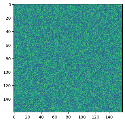
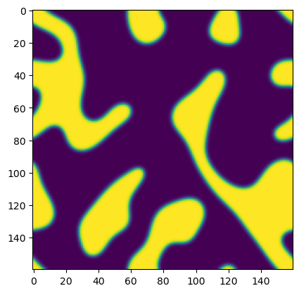
## Run an example simulation and plot the before and after
np.random.seed(0)
ic = np.random.random((160, 160)) - 0.5
model = AllenCahn(*ic.shape, kappa=1e1, d=1e-3)
tpts, sol = model.solve(ic, 0, 8, 400, method="DOP853")


plt.figure()
plt.imshow(sol[0], vmin=-1, vmax=1)

plt.figure()
plt.imshow(sol[-1], vmin=-1, vmax=1)
Running with Instructor Solutions. If you meant to run your own code, do not import from solutions
Sanity check: imaginary residual is: 6.181668750336787e-14
Additional information
In this example, we used first-order central finite differences in order to resolve the derivatives. Each finite-difference operation polls two lattice sites to compute a first derivative along a given direction, and it polls three lattice sites in order to compute a second derivative. If we have a very dense mesh and desire higher accuracy, we are free to use a higher-order approximation. On an uneven mesh, it may even make sense to adaptively choose the order of our operator based on the local lattice spacing.
Our example above is a simplified version of the Cahn-Hilliard equation, which is another model of phase separation with higher order terms in , leading to a rich range of dynamical behaviors such as spinodal decomposition and critical opalescence.
(Optional) We can try making a slider to visualize the time evolution of the field. This will require the ipywidgets package, which is not installed by default in Google Colab. If you are running this notebook in Google Colab, you can install the package by running !pip install ipywidgets in a code cell.
Turing’s model of morphogenesis and spectral methods
Reaction-diffusion equations are sets of partial differential equations describing interactions among multiple coupled fields. Reaction diffusion equations represent a protypical example of nonlinear partial differential equations where spatial effects give rise to unique bifurcations that cannot occur in similar ordinary differential equations.
Here, we are going to visit one of the most elegant known applications of reaction-diffusion dynamics: pattern formation. In 1952, Alan Turing used systems of reaction-diffusion equations to propose a model of morphogenesis: the process by which cheetahs get their spots, or leaves develop their unique shapes. While biological systems often give the impression that every detail of the patterns on a zebra or the plumage of a parrot is precisely programmed by an elaborate genetic circuit, Turing’s model suggests that two interacting chemical fields created early during the development of an organism can spontaneously produce surprisingly natural patterns, as long as natural selection has lead the governing parameters in the underlying equations to have just the right values.
The Gray-Scott model
The simplest example of reaction-diffusion equations producing Turing patterns is the Gray-Scott model, which describes a synthesis reaction between two chemical species and :
On a slower timescale, a second degradation reaction occurs in
Where is an inert byproduct of the reaction. During an organism’s development, the “slow” variable might represent a diffusing signalling molecule, while the fast reaction variable my represent the activity level of a gene activated by the molecule.
If this reaction occurs across a spatial domain, then we can write two scalar fields, and describing the concentrations of the two chemical species across space.
where and indicate separate diffusivities for the two reagents, and and parametrize autocatalysis of and degradation of , respectively. If and were two chemical species, then separate diffusivities might result from the two having very different molecular weights.
Spectral methods
Turing patterns have interesting mathematical structure because they reach steady-state solutions with nontrivial spatial heterogeneity in . This setting represents a perfect use case for a class of PDE solvers known as spectral methods, which seek to solve spatial PDEs in spatial frequency space rather than real space
The critical idea for spectral methods is to remember that the Fourier transform of the derivative of a function is proportional to a polynomial times the function in frequency space. Using the expanded notation for a Fourier transform , then and . These identities give us a way to transform our Gray-Scott equations into a more favorable representation; first by taking the Fourier transform of both sides of our equations, and then exploiting the linear properties of the Fourier transform operator. We can write our Gray-Scott equations in frequency space as
Where we have used to denote the respective Fourier transforms of and , . Hereafter, will use the condensed notation . Because we want to write these equations exclusively in terms of our frequency-space dynamical variables and , we re-write these equations as,
This is a bit of an ugly way to write things out, but it emphasizes the computational steps.
In the Fourier domain, we’ve gotten rid of the pesky Laplace operator that slowed down our integration in our previous problem. The tradeoff is that the reaction term looks more difficult now. In order to numerically integrate this equation in space, we would need to constantly convert between real and frequency space every time we want to compute the reaction term. Another option would be to convert back to real space,
We can see now the key idea behind spectral methods: at each timestep, we switch to whatever basis (real space or frequency space) that makes it easiest to evaluate the terms in our dynamical equations. If we’re working primarily in Fourier space, then we need to perform an inverse Fourier transform to calculate the real-space fields , calculate the reaction, and then convert back to Fourier space. If we are working in real space, we need to perform a Fourier transfom to get , calculate the diffusion term, and then perform an inverse Fourier transform to convert back to real space. If we were just solving an isolated diffusion equation, we could stay exclusively in Fourier space (likewise, real space for a purely reaction term). Unfortunately, we usually won’t get so lucky for many real-world PDEs.
Why would performing two Fourier transforms per timestep possibly be worthwhile compared to using the discrete Laplace operator, as we did above? While performing two fast Fourier transforms per timestep clearly increases the runtime per timestep, the key advantage of spectral methods is that they are usually very stable for long simulations. We can therefore decrease our mesh size (the number of spatial points in our domain), and still get a solution with the same accuracy. So, while using spectral methods increases the runtime of a single iteration of the right hand side for a given mesh size, we get time back because we can evaluate on a much coarser domain---for example, we might be able to go from a domain to a domain without losing much accuracy. For this reason, spectral methods can become particularly favorable in problems with many spatial dimensions.
To Do
Please complete the following tasks and answer the included questions. You can edit a Markdown cell in Jupyter by double-clicking on it. To return the cell to its formatted form, press [Shift]+[Enter].
Implement the Gray-Scott equations in Python, using the spectral method and the method of lines. I’ve included the outline of my solution below, but feel free to structure your code differently. Use periodic boundary conditions here, because the Fourier transform requires them. You will likely find the functions
np.fft.fft2()andnp.fft.ifft2()very useful here. There are several possible ways to solve this problem:(1) Purely in real space (it’s good practice not to use this approach here, since we already did it above for the Allen-Cahn model)
(2) Primarily in real-space, but switching to the Fourier domain and back within every call to the diffusion term.
(3) Primarily in the Fourier domain, but switching back-and-forth to real space every time within the reaction term. Remember to convert your final solution back to real space for visualizations.
Your Answer: Please fill in the code cells belowTry varying the parameters , and in your equations, and observe how the simulated solutions change. How do the solutions change? Do you have any intuition for why these changes might occur?
Your Answer: As mentioned above, performing Fourier transforms at each timestep is more expensive per mesh point than computing the discrete Laplacian at each timestep. Can you give a more mathematical reason for this advantage, based on runtime scaling of Fourier transforms? How many fewer mesh points would we need to compensate?
Your Answer: Try playing around with the number of timepoints and the number of space points. When does the spectral method fail? How do these failures differ from the ones we saw with the real-space finite difference scheme we used for the Allen-Cahn equations?
Your Answer: Evolutionary biologists recently showed strong evidence that the spacing of teeth-like denticles on sharks’ skin arises from a Turing mechanism. If we suppose that the denticles form via a Turing instability in Gray-Scott equations in early development, which parameter of the Gray-Scott equations would evolutionary forces most strongly act upon?
Your Answer: We assumed periodic boundary conditions, which makes this problem easier to implement. How do you expect our results would change, if we had Dirichlet boundary conditions?
Your Answer: from scipy.integrate import solve_ivp
class GrayScott:
"""
Simulate the two-dimensional Gray-Scott model
Parameters
nx (int): number of grid points in the x direction
ny (int): number of grid points in the y direction
Lx (float): length of the domain in the x direction
Ly (float): length of the domain in the y direction
du (float): diffusion coefficient for u
dv (float): diffusion coefficient for v
kappa (float): degradation rate of v
b (float): growth rate of u
"""
def __init__(self, nx, ny, du=0.1, dv=0.05, b=0.0545, kappa=0.1165, Lx=1.0, Ly=1.0):
self.nx, self.ny = nx, ny
self.dx = Lx / nx
self.dy = Ly / ny
self.du, self.dv = du, dv
self.kappa = kappa
self.b = b
## We need to define a mesh for the frequency domain
kx = (2 * np.pi / Lx) * np.hstack([np.arange(nx / 2 + 1), np.arange(1 - nx / 2, 0)]) / nx
ky = (2 * np.pi / Ly) * np.hstack([np.arange(ny / 2 + 1), np.arange(1 - ny / 2, 0)]) / ny
self.kx, self.ky = kx, ky
kxx, kyy = np.meshgrid(kx, ky)
ksq = kxx**2 + kyy**2
self.ksq = ksq
def _reaction(self, y):
"""
Compute the reaction term in real space
Args:
y (np.ndarray): array of shape (2 * nx * ny, ) containing the two fields
u and v, stacked together
"""
########################################################################
#
# Your code here. If you are performing the reaction in real space, this is
# relatively straightforward. If you are performing the reaction in Fourier
# space, you will need to perform an inverse Fourier transform
#
########################################################################
raise NotImplementedError
def _laplace(self, y):
"""
Calculate the Laplacian in Fourier space
"""
########################################################################
#
# Your code here.
#
########################################################################
raise NotImplementedError
def _diffusion(self, y):
"""
Calculate the diffusion term in Fourier space
Args:
y (np.ndarray): array of shape (2 * nx * ny, ) containing the two fields
u and v, stacked together
"""
########################################################################
#
# Your code here. I split the Laplace operator into its own function
#
########################################################################
raise NotImplementedError
def rhs(self, t, y):
"""
For technical reasons, this function needs to take a one-dimensional vector,
and so we have to reshape the vector back into the mesh
"""
########################################################################
#
# Your code here. This mainly calls other functions, in my implementation
#
########################################################################
raise NotImplementedError
def solve(self, y0, t_min, t_max, nt, **kwargs):
"""
Solve the heat equation using the solve_ivp solver
Args:
y0 (np.ndarray): initial condition
t_min (float): minimum time
t_max (float): maximum time
nt (int): number of time steps
**kwargs: keyword arguments to pass to solve_ivp
"""
########################################################################
#
# Your code here. I recommend using the solve_ivp solver, along with judicious
# use of np.reshape operation and np.hstack, because solve_ivp expects a
# one-dimensional vector as input
#
########################################################################
raise NotImplementedError
Test and use your code
You don’t need to write any code below, these cells are just to confirm that everything is working and to play with your sandpile implementation
If you are working from a local fork of the entire course, then you already have access to the solutions. In this case, make sure to
git pullto make sure that you are up-to-date (save your work first).If you are working from a single downloaded notebook, or are working in Google Colab, then you will need to manually download the solutions file from the course repository. The lines below will do this for you.
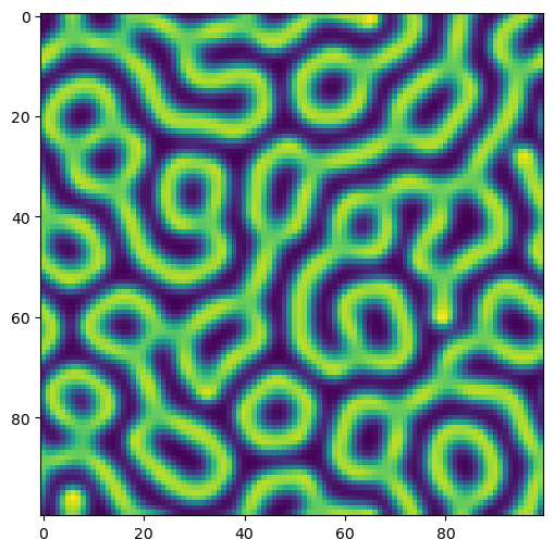
## Create initial conditions
np.random.seed(0)
u_ic = 0.5 +  1.5 * np.random.random((100, 100))
v_ic = 1 - np.copy(u_ic)

## Run simulation
model = GrayScott(*u_ic.shape)
tpts, sol = model.solve([u_ic, v_ic], 0, 5000, 500)

## Check that our spectral code is working: the imaginary residual should be small
print(f"Imaginary residual is: {np.mean(np.abs(np.imag(np.array(sol))))}")
sol = np.real(sol)

plt.figure(figsize=(6, 6))
plt.imshow(sol[-1, ..., 1])
Running with Instructor Solutions. If you meant to run your own code, do not import from solutions
Imaginary residual is: 0.0
(optional) Make an interactive video with a slider in the notebook. This will require the ipywidgets package, which is not installed by default in Google Colab. If you are running this notebook in Google Colab, you can install the package by running !pip install ipywidgets in a code cell.
## Create an interactive plot using ipywidgets

from ipywidgets import interact, interactive, fixed, interact_manual, Layout
import ipywidgets as widgets

def plotter(i):
    fig = plt.figure(figsize=(10, 10))
    plt.imshow(sol[i, ..., 1])
    plt.show()


interact(
    plotter,
    i=widgets.IntSlider(0, 0, len(sol) - 1, 1, layout=Layout(width='500px'))
)<function __main__.plotter(i)>Additional information
Our trick of switching the equations to the frequency might not seem that satisfying---we made the diffusion term easier to solve, but at the expense of having to round-trip the reaction term between real space and frequency space at every timestep. Deciding between real space and frequency space for a numerical integration problem is very context specific---here, we could guess that spectral methods are preferable because (1) periodic boundary conditions, (2) symmetry considerations, and (3) our simple reaction term. It turns out that, for many reaction-diffusion systems, there’s a way to avoid converting the reaction term at each timestep, through clever use of integrating factors.
You likely noticed that we glazed over the issue of boundary conditions. Projecting the PDE onto a Fourier basis implicitly assumes that we are working on a toroidal domain. Spectral methods include many options beyond just Fourier transforms. For Dirichlet boundary conditions, we can use Chebyshev polynomials as our basis functions instead.
We saw that the Fourier domain was a natural setting for reaction-diffusion problems. Analytical tools for predicting Turing patterns confirm the appearance of patterns corresponds to an instability where one frequency component grows exponentially at the expense of all of the others---if we think of the system as a set of coupled ODEs repesenting different spatial frequencies, the instability corresponds to a solution where one variable diverges, while all the others go to zero. These diffusion-driven instabilities are explored in Chapter 2 of Murray Mathematical biology.
The biological accuracy of Turing’s model remains a topic of research, but the reaction-diffusion model has been experimentally-tested and even directly manipulated in certain specific systems---including angelfish patterns, shark skins, bird feathers, and lizard skins.
Depending on their parameters, single-component diffusion-like equations like the Allen-Cahn equations can produce travelling, soliton-like fronts, which have been used to describe everything from epidemic spread, to propogation of beneficial genetic mutations, to
Dedalus is an excellent new Python library for solving PDEs with spectral methods. The earlier MATLAB library chebfun has a similar purpose.
Optional Exercises
Compare runtime scaling for different meshes and timesteps, for both spectral and finite-difference methods. At what lattice sizes does it make sense to use real-space versus spectral methods?
Like a bifurcation in a system of ODEs, it is possible to compute the analytical bifurcation threshold for diffusion-driven instability in the Gray-Scott equations, compared to when the numerics show bifurcation. The two should agree when the mesh is sufficiently fine.
- Cooper, R. L., Thiery, A. P., Fletcher, A. G., Delbarre, D. J., Rasch, L. J., & Fraser, G. J. (2018). An ancient Turing-like patterning mechanism regulates skin denticle development in sharks. Science Advances, 4(11). 10.1126/sciadv.aau5484