Preamble: Run the cells below to import the necessary Python packages

import numpy as np

# Wipe all outputs from this notebook
from IPython.display import Image, clear_output, display
clear_output(True)

# Import local plotting functions and in-notebook display functions
import matplotlib.pyplot as plt
%matplotlib inline
Revisiting the coauthorship graph
We previously considered the coauthorship graph among physicists based arXiv postings in astro-ph. The graph contains nodes, which correspond to unique authors observed over the period 1993 -- 2003. If Author i and Author j coauthored a paper during that period, their nodes are connected. In order to analyze this large graph, we will downsample it to a smaller graph with nodes representing the most highly-connected authors.
This dataset is from the Stanford SNAP database
import io
import gzip
import urllib.request
import networkx as nx

# subject = "CondMat"
# subject = "HepPh"
# subject = "HepTh"
# subject = "GrQc"
subject = "AstroPh"
url = f"https://snap.stanford.edu/data/ca-{subject}.txt.gz"

with urllib.request.urlopen(url) as resp:
    with gzip.open(io.BytesIO(resp.read()), mode="rt") as fh:
        g = nx.read_edgelist(fh, comments="#", nodetype=int)
## Create a subgraph of the 1000 most well-connected authors
subgraph = sorted(g.degree, key=lambda x: x[1], reverse=True)[:4000]
subgraph = [x[0] for x in subgraph]
g2 = g.subgraph(subgraph)
# rename nodes to sequential integers as they would appear in an adjacency matrix
g2 = nx.convert_node_labels_to_integers(g2, first_label=0)
pos = nx.spring_layout(g2)
# pos = nx.kamada_kawai_layout(g2)
# nx.draw_spring(g2, pos=pos, node_size=10, node_color='black', edge_color='gray', width=0.5)
nx.draw(g2, pos=pos, node_size=5, node_color='black', edge_color='gray', width=0.5, alpha=0.5)
plt.show()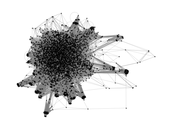
Estimating degree distributions, centrality, and the PageRank algorithm
We previously saw that the degree distribution determines how often a random walk on the graph will visit a given node. This can be seen an an indicator of how “important” a given node is to the structure of the graph. If we wanted to rank the authors purely based on their degree distribution, we could write this ranking as
where is a vector of ones, is our adjacency matrix, and is our desired ranking. Notice how the matrix product with the ones vector allows us to compute the rowwise sum. This makes sense, because we expect that this operation should take operations, and matrix-vector products are .
A = nx.adjacency_matrix(g2).todense() # get the binary adjacency matrix of the graph
rank_degree = A @ np.ones(A.shape[0])
plt.figure(figsize=(7, 7))
nx.draw(g2, pos=pos, node_size=200, node_color=np.log10(rank_degree), edge_color='gray', width=0.01, cmap='viridis', alpha=0.2)
plt.title(f"Authors ranked by degree")
plt.show()
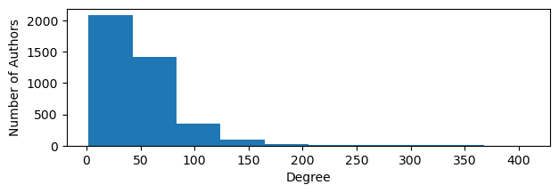
plt.figure(figsize=(7, 2))
plt.hist(rank_degree)
plt.ylabel("Number of Authors")
plt.xlabel("Degree")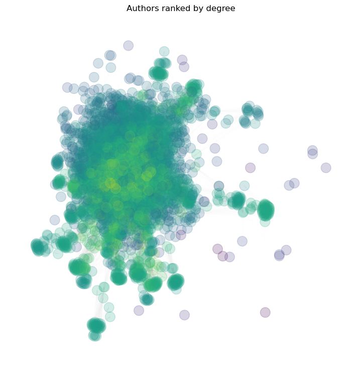
How else might we group authors?
The degree ranking simply tells use who are the most well-connected authors are. They are the individuals who directly co-authored a paper with someone else at any point during the period over which the arXiv dataset was collected.
Recall that we can think of the degree distribution as the long-time limit of a random walker that “hops” among the neighboring nodes in a graph. What if we add stochasticity? What if we allow the random walker to sometimes jump to any new node, not connected to the current node? This will cause the walker to explore the graph more broadly, and discover authors who are less connected to the dominant central cluster. We will draw a loose analogy with the Ornstein-Uhlenbeck process. The spring constant pulls a random walker back to the origin, but the random noise allows the walker to explore the space more broadly. Likewise, the degree distribution pulls the random walker to the most connected nodes, but random jumps allow the walker to explore the graph more broadly.
This is the idea behind the PageRank algorithm, which is how Google originally ranked web pages. In Google’s case, the entire internet is too large to know a priori the adjacency matrix of all web pages. Instead, they use a random walk algorithm to estimate the degree distribution of the web pages. Random hops allow the algorithm to more easily find smaller subnetworks, so that it doesn’t keep revisiting dominant nodes like Wikipedia or Facebook. This is sometimes refered to as the “random surfer model” of PageRank.
Implementing the PageRank algorithm
We are now going to implement the PageRank algorithm on the coauthorship graph. The PageRank algorithm is a variant of the random walk algorithm that allows the random walker to sometimes jump to a new node with probability .
If we interpret our desired ranking as a probability distribution, then we can write a master equation describing the dynamics of the probability distribution of many random walkers. The vector represents the unnormalized probability distribution of the random walkers at time , and so we refer to it as the “rank” because its relative values, but not absolute values, represent the relative importance of a given node.
where is a vector of ones, is the adjacency matrix of the graph, and is a parameter that controls the probability of the random surfer jumping to a random node. The first term on the right-hand side represents the process of the walker moving to a neighboring node, while the second term represents the process of jumping to a new node.
Solving this equation for the steady state distribution results in the PageRank equation
This equation can be rewritten as an equation for ,
where is the identity matrix. We write these equations as a single matrix equation
where . If we set (no random jumps), then this equation becomes
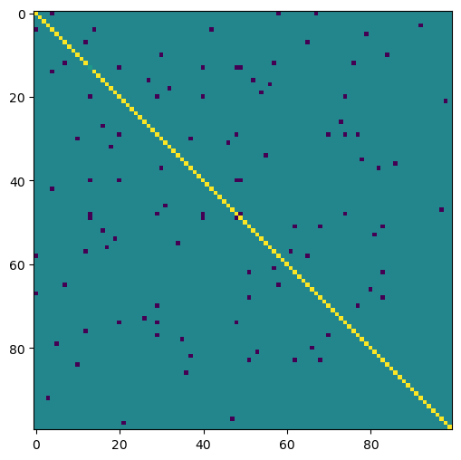
alpha = 0.85 # a typical damping factor used in PageRank
M = (1 - alpha) * (np.eye(A.shape[0]) - alpha * A)
print(M.shape)

plt.figure(figsize=(6, 6))
plt.imshow(M[:100, :100])
(4000, 4000)
Inverting a matrix
So far, we have taken for granted that we can easily invert a large matrix . Given a linear problem
with , , and , we can solve for by inverting :
How would we do this by hand?
Gauss-Jordan elimination: perform a series of operations on both the left and the right hand sides of our equation (changing both and ), until the left side of the equation is triangular in form. Because Gauss-Jordan elimination consists of a series of row-wise addition and subtraction operations, we can think of the process as writing each row vector in terms of some linear combination of row vectors, making the whole process expressible as a matrix
where we have defined the upper-triangular matrix . This confirms our intuition that the time complexity of Gauss-Jordan elimination is , since that’s the time complexity of multiplying two matrices.
Why do we want triangular matrices?
If we can reduce our matrix to upper-triangular form, then we can quickly solve for using forward substitution. This should take operations if
We can implement a forward substitution algorithm that takes advantage of the fact that the matrix is triangular. To simplify our notation, we will assum that is lower-triangular, so that the first row has only one non-zero element at . We can theniterate over rows of in order to find the elements of the solution vector one-by-one. For example, the first element is simplygiven by
The second element is given by
and so on. We can therefore write a general algorithm for forward substitution as
Notice how the number of operations scales with the number of non-zero elements in the row. We can apply the same approach to an upper-triangular matrix, but we would need to iterate over the rows in reverse order.
def solve_tril(a, b):
    """
    Given a triangular matrix, solve using forward subtitution

    Args:
        a (np.ndarray): A lower triangular matrix
        b (np.ndarray): A vector

    Returns:
        x (np.ndarray): The solution to the system
    """
    n = a.shape[0]
    x = np.zeros(n)
    for i in range(n):
        x[i] = (b[i] - np.dot(a[i, :i], x[:i])) / a[i, i]
    return x

## Make a random lower triangular matrix
a = np.tril(np.random.random((10, 10)))
b = np.random.random(10)

## Using built-in solver
print(np.linalg.solve(a, b))

## Using our implementation
print(solve_tril(a, b))

# Check that the numpy and our implementation give the same result
print(np.allclose(np.linalg.solve(a, b), solve_tril(a, b)))
# print(np.all(np.linalg.solve(a, b) == solve_tril(a, b)))
# np.sum(np.abs(np.linalg.solve(a, b) - solve_tril(a, b))) < 1e-14
[  2.81351726  -2.8605426    3.42947717   0.12737231  -4.40757578
  -8.52289754   6.82569524  37.08546637 -27.81740643 -15.54479122]
[  2.81351726  -2.8605426    3.42947717   0.12737231  -4.40757578
  -8.52289754   6.82569524  37.08546637 -27.81740643 -15.54479122]
True
Looking at our implementation of the triangular solve, we can see that it has a single for loop over the rows of the matrix. However, within each row, it performs a dot product. In the first row, this dot product reduces to a single scalar multiplication, but in the final row, it reduces to a dot product of elements. Across the steps of the for loop, the number of product-sum operations, on average, is proportional to .
Across the explicit outer loop and the vectorized dot product, we therefore expect to perform operations total. Another way to see this is that the number of operations is proportional to the number of non-zero elements in the matrix, which is for a lower-triangular matrix.
Let’s see if this scaling holds in practice by using the timeit module to see how the runtime of our implementation scales with the matrix size. We will compare our implementation to the built-in numpy solver.
import timeit

all_times1, all_times2 = list(), list()
nvals = np.arange(10, 500)
for n in nvals:
    ## Upper triangular solve
    a = np.tril(np.random.random((n, n)))
    b = np.random.random(n)
    all_reps = [timeit.timeit("solve_tril(a, b)", globals=globals(), number=10) for _ in range(10)]
    all_times1.append(np.mean(all_reps))

    # ## Full solve with numpy
    all_reps = [timeit.timeit("np.linalg.solve(a, b)", globals=globals(), number=10) for _ in range(10)]
    all_times2.append(np.mean(all_reps))

plt.loglog(nvals, all_times1, label="Triangular solve")
plt.loglog(nvals, all_times2, label="Full solve")
plt.loglog(nvals, 1e-6 * nvals**2, "--", label="Quadratic Scaling")
plt.xlabel("Matrix size")
plt.ylabel("Time (s)")
plt.legend(frameon=False)
plt.show()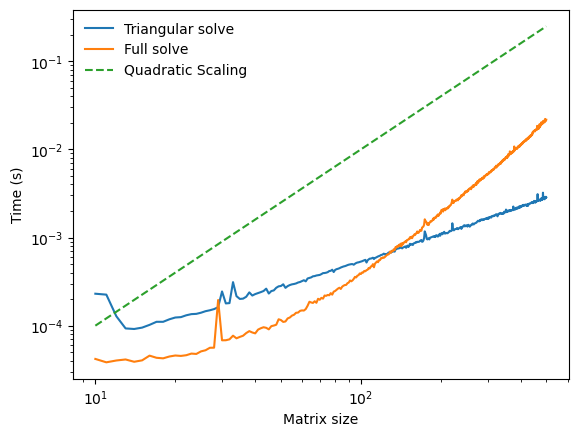
The scaling does not match our expectation. We can see that the empirical scaling almost looks like for our triangular solver. But we know that this is physically impossible, because we have to access non-zero elements in to solve the system.
What happened? Timescale separation between our nested operations. The outer for loop is written in Python, which is slow, but the inner dot product is vectorized, and so it uses the highly optimized BLAS library. As a result, the inner loop is much faster than the outer loop, and so we don’t see the quadratic scaling at these matrix sizes. In fact, in order to see the quadratic scaling, we would need to access matrix sizes that are so large that we would run out of memory on a typical computer. So, in this case, we are not able to perform numerical experiments that reach the true asymptotic scaling regime.
What about numpy’s built-in solver? It performs way faster than our solver at small matrix sizes, but it appears to gets much worse as the matrix gets larger. This is because, unlike our implementation, numpy’s solver applies to any square matrix. It does not know in advance that our matrix has exploitable triangular structure, and the time cost to check for this structure before solving is substantial enough that it is better for to use a general solver instead. General matrix inversion has the same time complexity as Gauss-Jordan elimination or matrix-matrix multiplication, which is . However, various advanced algorithms have been developed that drive down the prefactor.
Exploiting sparsity. We can see that triangular solvers are a specific case of a common phenomenon in numerical linear algebra. If a matrix has particular structure, particularly sparsity, the time cost of many operations can be reduced to be proportional to the number of nonzero elements. Since a triangular matrix has nonzero elements, it’s worth exploiting this structure when performing a operation like matrix inversion.
To invert a full matrix, we first need reach triangular form
We know that we want to modify our full matrix equation
using a Gauss-Jordan elimination procedure, which we know has the form of a matrix multiplication
We define , and we know that if can reduce to upper-triangular form, then we can solve for using forward substitution in operations.
But what is the form of ?
Our key insight is that the Gaussian elimination matrix for a full matrix inversion turns is a triangular matrix. Moreover, because the inverse of a triangular matrix is also a triangular matrix (this can be shown by writing out the algebraic terms in the matrix multiplication algebra for ), we therefore write a transformed version of our problem
defining , we arrive at the celebrated LU matrix factorization
where is a lower triangular matrix, and is an upper triangular matrix.
We can therefore solve for by introducing an intermediate variable , and then
If we can find the LU form, exactly solving the linear problem consists of two steps, each of which has a time complexity of :
Solve the equation . Since is a triangular matrix, this can be performed using substitution
Solve the equation . Since is also triangular, this inverse can also be computed using substitution
The hard part, then, will be to find the LU form in the first place. This is equivalent to finding the Gaussian elimination matrix for the full matrix inversion problem.
About LU factorization
An iterative implementation of factorization uses Gauss-Jordan elimination in a principled order. We first eliminate the first column of the matrix, then the second column, and so on. A more sophisticated algorithm, Crout’s method with pivoting, performs optimal order of decomposition based on the specific values present in a given row or column. However, our approach is matrix agnostic, and so we will not implement pivoting.
Decomposition into L and U is for an matrix, meaning that it has the same time complexity as matrix-matrix multiplication.
Given a matrix and target , what is the overall runtime to find ?
The LU decomposition algorithm
Set and (the input matrix)
For each column in :
Choose the pivot element , corresponding to the diagonal element in the column
For each row below the pivot:
Find the multiplier
Subtract the entire th row from the row in
Store in the row of
In the context of the LU decomposition algorithm, the ‘pivot’ refers to the element in the current column, denoted as , that we are processing in the outer loop. The pivot serves as a divisor to find the multipliers which are then used to eliminate the elements below the pivot, making them zero to carve out an upper triangular matrix .
Simultaneously, these multipliers are stored in the lower triangular matrix . Essentially, we are utilizing the pivot to find scalar values that can help perform row operations to systematically zero out elements below the diagonal in , while building up the matrix. We can see that there are three nested loops, which means that the time complexity of the LU decomposition algorithm is .
class LinearSolver:
    """
    Solve a linear matrix equation via LU decomposition (naive algorithm)
    """
    def __init__(self):
        # Run a small test upon construction
        self.test_lu()

    def lu(self, a):
        """Perform LU factorization of a matrix"""
        n = a.shape[0]
        L, U = np.identity(n), np.copy(a)
        for i in range(n):
            factor = U[i+1:, i] / U[i, i] # the multiplier for the current row
            L[i + 1:, i] = factor
            U[i + 1:] -= factor[:, None] * U[i]
        return L, U

    # A unit test of a single class method
    def test_lu(self):
        """A small test method that the factorization is correct"""
        X = np.random.random((10, 10))
        L, U = self.lu(X)
        assert np.allclose(X, L @ U), "LU decomposition failed"

    def forward_substitution(self, L, b):
        """Solve a lower triangular matrix equality of the form Lx = b for x"""
        n = L.shape[0]
        y = np.zeros(n)
        y[0] = b[0] / L[0, 0]
        for i in range(1, n):
            y[i] = (b[i] - np.dot(L[i,:i], y[:i])) / L[i,i]
        return y

    def backward_substitution(self, U, b):
        """Solve an upper triangular matrix equality of teh form Ux = b for x
        NOTE: replace with second call to forward and a transposition operation
        """
        n = U.shape[0]
        y = np.zeros(n)
        y[-1] = b[-1] / U[-1, -1]
        for i in range(n-2, -1, -1):
            y[i] = (b[i] - np.dot(U[i,i+1:], y[i+1:])) / U[i,i]
        return y

    def solve(self, X, b):
        L, U = self.lu(X)
        self.L, self.U = L, U

        # Intermediate variable
        h = self.forward_substitution(L, b)

        return self.backward_substitution(U, h)


# Construct a random linear problem
A = np.random.rand(4, 4)
b = np.random.rand(4)

# My implementation
model = LinearSolver()
print(model.solve(A, b))

# Solve the linear problem using the numpy built-in solver
print(np.linalg.solve(A, b))

print(np.allclose(model.solve(A, b), np.linalg.solve(A, b) ))
[-3.05699723e+00 3.46713239e+00 -1.31202253e-03 1.20541708e+00]
[-3.05699723e+00 3.46713239e+00 -1.31202253e-03 1.20541708e+00]
True
Applying LU Decomposition of orthogonal basis sets
A Hadamard matrix is a square matrix comprising a complete collection of length mutually-orthogonal vectors with all elements equal to either +1 or -1. We can convert any complete orthonormal basis to a Hadamard matrix by ordering the vectors systematically, and substituting 0 and 1 for with a recursive rule. The recursive rule to generate a Hadamard matrix is
where the base case is . We can build this matrix bottom-up using dynamic programming, or top-down using recursion.
def hadamard(n):
    """
    Create a Hadamard matrix of size n using recursion
    """
    if n == 1:
        return np.array([[1]])
    else:
        H = hadamard(n // 2)
        return np.block([[H, H], [H, -H]])

def hadamard(n):
    """
    Create a Hadamard matrix of size n using dynamic programming
    """
    H = np.array([[1.]])
    for i in range(int(np.log2(n))):
        H = np.block([[H, H], [H, -H]])
    return H

plt.figure(figsize=(8, 8))
a = hadamard(2**8).astype(float)
plt.imshow(a, cmap='gray')
plt.axis('off')
(np.float64(-0.5), np.float64(255.5), np.float64(255.5), np.float64(-0.5))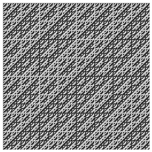
We can verify that the Hadamard matrix is orthogonal by computing its condition number, .
np.linalg.cond(a)np.float64(1.0000000000000024)Since all rows and columns have inner product zero with each other, the matrix is orthogonal, and so the condition number is the lowest possible value of 1. Recall that the condition number of a random matrix is .
We can see that the Hadamard matrix has unique structure due to its self-similar construction. We can highlight this structure by decomposing the Hadamard matrix into its and factors.
ll, uu = model.lu(a)

plt.figure(figsize=(9, 4.5))
plt.subplot(121)
plt.imshow(ll, cmap='gray')
plt.axis('off')
plt.subplot(122)
plt.imshow(uu.astype(bool), cmap='gray')
plt.axis('off')
## show plots closer together
plt.subplots_adjust(wspace=0.1)
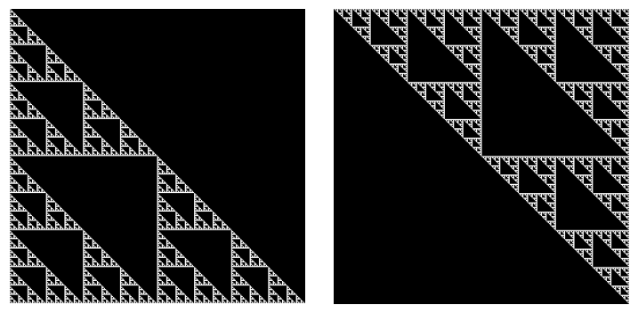
We can see that the and matrices are both fractal matrices known as the Sierpinski triangle.
Applying PageRank to the coauthorship graph
Now that we have a method for inverting a matrix, we can now apply the PageRank algorithm to the coauthorship graph. Recall that the PageRank algorithm is a random walk algorithm that can be written as a matrix inversion problem:
where .
A = nx.adjacency_matrix(g2).todense() # get the binary adjacency matrix of the graph

def find_pagerank(A, alpha=0.85, verbose=False):
    """
    Find the PageRank of a graph using matrix inversion

    Args:
        A (np.ndarray): The adjacency matrix of the graph
        alpha (float): The damping factor. The default value is 0.85

    Returns:
        page_rank (np.ndarray): The PageRank of each node
    """
    M = (1 - alpha) * (np.eye(A.shape[0]) - alpha * A)

    if verbose:
        print(f"Condition number of M: {np.linalg.cond(M)}", flush=True)

    ## use our LU solver to solve for the PageRank
    # page_rank = np.linalg.inv(M) @ np.ones(M.shape[0])
    l, u = LinearSolver().lu(M)
    Minv = np.linalg.inv(u) @ np.linalg.inv(l)
    page_rank = Minv @ np.ones(M.shape[0])

    return page_rank

plt.figure(figsize=(8, 3))

## We plot the degree distribution (equivalent to alpha=1.0)
plt.subplot(131)
nx.draw(g2, pos=pos, node_size=200, node_color=np.log10(rank_degree),
        edge_color='gray', width=0.02, cmap='viridis', alpha=0.2)
plt.title(f"alpha=1.00")

## PageRank distribution with alpha=0.99
plt.subplot(132)
page_rank2 = find_pagerank(A, alpha=0.99, verbose=True)
nx.draw(g2, pos=pos, node_size=200, node_color=np.log10(page_rank2),
        edge_color='gray', width=0.02, cmap='viridis', alpha=0.2)
plt.title(f"alpha=0.99")

## PageRank distribution with alpha=0.05
plt.subplot(133)
page_rank1 = find_pagerank(A, alpha=0.05, verbose=True)
nx.draw(g2, pos=pos, node_size=200, node_color=np.log10(page_rank1),
        edge_color='gray', width=0.02, cmap='viridis', alpha=0.2)
plt.title(f"alpha=0.05")
/var/folders/79/zct6q7kx2yl6b1ryp2rsfbtc0000gr/T/ipykernel_56959/1688625460.py:45: RuntimeWarning: invalid value encountered in log10
nx.draw(g2, pos=pos, node_size=200, node_color=np.log10(page_rank2),
/var/folders/79/zct6q7kx2yl6b1ryp2rsfbtc0000gr/T/ipykernel_56959/1688625460.py:52: RuntimeWarning: invalid value encountered in log10
nx.draw(g2, pos=pos, node_size=200, node_color=np.log10(page_rank1),
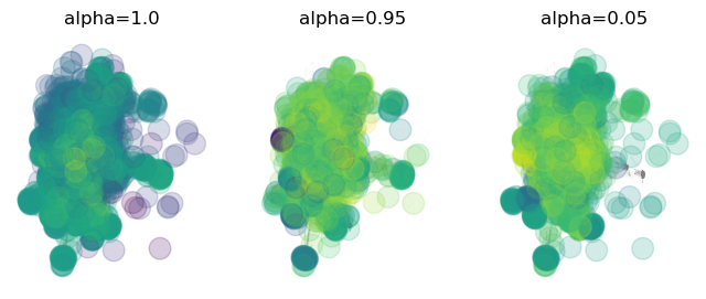
We can see that high values of cause the PageRank algorithm to look more like the degree distribution. This emphasizes larger subnetworks and and more highly-connected nodes. Conversely, low values of cause the PageRank algorithm to converge to something closer to a uniform distribution over all nodes. The effect of the damping factor is to control the trade-off between the random walk limit, which samples the well-connected nodes better, and the limit in which all nodes are sampled with equal probability. The latter case helps sample rarer nodes more frequently, at the expense of accurately representing the degree distribution for higher-degree nodes.