Numerical integration and extinction rates in large random ecosystems

Requirements

matplotlib
numpy
scipy

A note on cloud-hosted notebooks. If you are running a notebook on a cloud provider, such as Google Colab or CodeOcean, remember to save your work frequently. Cloud notebooks will occasionally restart after a fixed duration, crash, or prolonged inactivity, requiring you to re-run code.

import numpy as np
import matplotlib.pyplot as plt
%matplotlib inline

Image from Tom Bech, CC BY 3.0 https://creativecommons.org/licenses/by/3.0, via Wikimedia Commons

The Lotka-Volterra model¶

The Lotka-Volterra model is a simple model of predator-prey interactions in a complex ecosystem. It is given by a system of coupled differential equations,

\frac{dn_i(t)}{dt} = n_i(t) \left( r_i + \sum_{j=1}^N A_{ij} n_j(t) - d_i n_i(t)\right)

(1)

where $n_i(t)$ is the number of individuals of species $i$ at time $t$ , $r_i > 0$ is the intrinsic population growth rate of species $i$ , $d_i > 0$ is a population-limitation constant such as overcrowding or resource scarcity, that prevents species $i$ from continuing to grow in number indefinitely. The term $A_{ij}$ is the interaction coefficient between species $i$ and $j$ . The matrix $A$ is assumed to be traceless ( $A_{ii}=0$ for all $i$ ), because the terms $r_i$ and $d_i$ cover the self-terms already. If $A_{ij} > 0$ , then species $i$ benefits from the presence of species $j$ , such as through symbiotic interactions, and if $A_{ij} < 0$ , then species $i$ is harmed by the presence of species $j$ , such as by predation. If $A_{ij} = 0$ , then species $i$ and $j$ do not directly interact, though they may indirectly interact through other species. The total number of species is given by $N$ , and so we have $N$ equations, one for each species.

A single species¶

We can understand the behavior of Eq. (1) by first considering the case where $N=1$ , in which case the dynamics become a one-dimensional ordinary differential equation,

\frac{dn_1}{dt} = n_1 \left( r_1 - d_{1} n_1 \right)

(2)

We may recognize that this equation defines sigmoidal growth dynamics, with exact solution given by the logistic growth curve,

n_1(t) = e^{r_1 t} \frac{n_1(0)}{r + n_1(0)(e^{r_1 t} - 1) d_1}

(3)

When $n_1$ or $d$ are small, the population grows exponentially. However, at long times, the overcrowding term, $d_1$ causes the population density to reach an asymptote $N_\text{max} = r_1/d_1$ , known in ecology as the carrying capacity of the population. The logistic growth curve is sometimes reparameterized in terms of this parameter.

Predator-prey dynamics¶

Another well-known specific case of Eq. 1 is predator-prey dynamics when $N=2$ . In this case, the model is given by

\frac{dn_1}{dt} = -n_1 \left( r_1 + A_{12} n_2 \right)

(4)

\frac{dn_2}{dt} = n_2 \left( r_2 - A_{21} n_1 \right)

(5)

For the specific case of predator-prey interactions, we set the signs and assume all of the parameters $r_i$ , $A_{ij}$ are positive. Notice that $n_1$ , the predator, has a negative growth rate, and so it decreases in population in the absence of prey. However, by encountering and eating the prey (the cross-term), it can increase its population. Conversely, $n_2$ describes the prey, which can graze or forage to increase its population in the absence of predators ( $r_2 > 0$ ). However, interactions with the predator reduce the prey population.

When the interactions are balanced, the predator and prey populations will oscillate: the prey population initially increases, which causes the predator population to increase with a delay. However, as the predator population increases, it will consume more prey, which causes the prey population to decrease. This, in turn, causes the predator population to decrease, and the cycle repeats. These dynamics have previously been observed in real ecosystems containing few species, such as the dynamics of lynxes and hares in the Canadian wilderness.

Random ecosystems¶

What do we expect for the dynamics of the predator-prey model in the limit of large ecosystems ( $N \to \infty$ )? Experimentally, each term in the species interaction matrix $A_{ij}$ requires isolating a pair of species, and measuring how they interact. Additionally, measuring the intrinsic growth and saturation rates $r_i$ , $d_i$ requires an additional set of $N$ isolation experiments, for a total of $N(N+1)$ total experiments in order to pin down the values of every parameter in Eq. 1. This may be feasible in the case of lynxes and hares, but it becomes more fraught for systems like the gut microbiome ( $N \sim 10^3$ species) or a coral reef ( $N \sim 10^6$ species).

In the spirit of May’s work, we are therefore going to study the behavior of Eq. 1 when all of the parameters are drawn from random distributions: $r_i \sim \mathcal{N}(0, 1)$ , $A_{ij} \sim \mathcal{N}(0, 1)$ . Physically, that means that we assume an ecosystem with a roughly equal number of mutualistic and antagonistic interactions, and we assume that equal numbers of species grow or die out in isolation, much like the lynxes and hares. Importantly, the interactions $A$ can be non-reciprocal: the effect of species $i$ in the growth rate of species $j$ may not be the same as the effect of species $j$ in the growth rate of species $i$ , and so $A_{ij} \neq A_{ji}$ in general (the predator prey case above is a good example of a strongly non-reciprocal system.

To Do¶

Please complete the following tasks and answer the included questions. You can edit a Markdown cell in Jupyter by double-clicking on it. To return the cell to its formatted form, press [Shift]+[Enter].

Implement the random Lotka-Volterra model Eq. 1. We will numerically integrate this system using the built-in scipy ODE solver scipy.integrate.solve_ivp with the integration method RK45 (the embedded method Runge-Kutta 4(5)).

    Your Answer: complete the code below

We can accelerate the simulation by using a more efficient method. Implicit methods allow larger timesteps or more accurate updates, by inverting the Jacobian (a locally linear approximation of the dynamics) at each timestep. Recall that, for a system of ODEs, the Jacobian is given by the matrix of partial derivatives of the right-hand side of the equations with respect to the each of the state variables. Calculate the analytic jacobian of the Lotka-Volterra model, and then use it to implement an implicit method. This will allow us to instead use the built-in scipy ODE solver scipy.integrate.solve_ivp with the implicit integration method Radau.

    Your Answer: complete the code below

One interesting phenomenon you will observe is that not all species survive at equilibrium, which we define as a species having a number of individuals less than our precision floor as $t \to \infty$ . Explore what happens when you run the simulation many times. Plot the final distribution of population sizes. What does this distribution resemble? What would you expect the distribution of population sizes to look like if there were no interactions ( $A_{ij}=0$ , $i\neq j$ )? What would you expect the distribution of population sizes to look like if we instead sampled from a distribution of interactions that is not centered at zero? Hint: you will find that the analytic results of Servan et al. 2018 confirm your numerical observations.

    Your Answer:

Suppose that, instead of sampling from the normal distribution, we instead sampled from a heavy-tailed distribution (a distribution with more very large values). How would you expect this to affect the dynamics of the system? You can try estimating this by modifying your simulation, or based on your intuition for the dynamics of the system. Hint: the steady-state, $\lim_{t\to\infty} n(t)$ , is not the only thing that might change.

    Your Answer:

from scipy.integrate import solve_ivp

class LotkaVolterra:
    """
    An implementation of the Lotka-Volterra model

    Parameters:
        n (int): number of species
        sigma (float): the scale of the randomly-sampled elements, Defaults to 1.0
        d (float): the density-limitation strength. Defaults to 10.0

    """

    def __init__(self, N, sigma=1.0, d=12.5, random_state=None):
        ################################################################################
        #
        #
        #  YOUR CODE HERE
        #  The instructor solution is ten lines and uses np.random.normal() and 
        #  np.random.seed()
        #
        #
        ################################################################################
        # raise NotImplementedError("Implement this method")

        self.N = N
        self.sigma = sigma
        self.random_state = random_state
        np.random.seed(self.random_state)
        ## Create a hollow random matrix
        self.r = np.random.normal(size=(self.N,), scale=self.sigma)
        self.A = np.random.normal(size=(self.N, self.N), scale=self.sigma)
        self.A = self.A - np.diag(self.A)
        self.d = d


    def rhs(self, t, n):
        """
        Given a time and a state vector, return the right-hand side of the Lotka-Volterra equations
        """
        ################################################################################
        #
        #
        #  YOUR CODE HERE
        #  The instructor solution is one line
        #
        #
        ################################################################################
        # raise NotImplementedError("Implement this method")

        return n * (self.r + np.dot(self.A, n) - self.d * n)
    

class LotkaVolterraWithJacobian(LotkaVolterra):
    """
    A subclass of the Lotka-Volterra model that adds a Jacobian functions
    """

    def __init__(self, *args, **kwargs):
        super().__init__(*args, **kwargs)

    def jacobian(self, t, n):
        """
        Given a time and a state vector, return the Jacobian of the Lotka-Volterra equations
        """
        ################################################################################
        #
        #
        #  YOUR CODE HERE.
        #
        #
        ################################################################################
        # raise NotImplementedError("Implement this method")
        # return np.diag(self.r + np.dot(self.A, n)) + self.A * n[:, None] - self.d * n
        # g = self.r + np.dot(self.A, n) - self.d * n
        # return np.diag(g) + np.diag(n) @ (self.A - np.diag(self.d))
        A2 = self.A - self.d * np.eye(self.N)
        return np.diag(self.r + np.dot(A2, n)) + A2 * n[:, None]

Test and use your code¶

You don’t need to write any code below, these cells are just to confirm that everything is working and to play with your implementation
If you are working from a local fork of the entire course, then you already have access to the solutions. In this case, make sure to git pull to make sure that you are up-to-date (save your work first).
If you are working from a single downloaded notebook, or are working in Google Colab, then you will need to manually download the solutions file from the course repository. The lines below will do this for you.

import os
import requests
# Check if the "solutions" directory exists. If not, create it and download the solution file
if not os.path.exists('solutions'):
    os.makedirs('solutions')
else:
    print('Directory "solutions" already exists. Skipping creation.')

# Now download the solution file into the directory we just created
url = 'https://raw.githubusercontent.com/williamgilpin/cphy/main/hw/solutions/allencahn_spectral.py'
response = requests.get(url)
file_path = os.path.join('solutions', 'sandpile.py')
with open(file_path, 'wb') as file:
    file.write(response.content)
print(f'File saved to {file_path}')
# Now download the solution file into the directory we just created
url = 'https://raw.githubusercontent.com/williamgilpin/cphy/main/hw/solutions/allencahn.py'
response = requests.get(url)
file_path = os.path.join('solutions', 'sandpile.py')
with open(file_path, 'wb') as file:
    file.write(response.content)
print(f'File saved to {file_path}')

## Initialize simulation parameters
N = 200
lv = LotkaVolterra(N, random_state=0)
# initial population sizes of all species should be greater than one
n0 = 0.2 * np.random.uniform(size=(N,))
sol = solve_ivp(lv.rhs, [0, 1000], n0, method="RK45")
plt.figure(figsize=(7, 5))
plt.semilogx(sol.t, sol.y.T);
plt.xlabel("Time")
plt.ylabel("Population sizes")
plt.title("Lotka Volterra Dynamics with Runge-Kutta solver")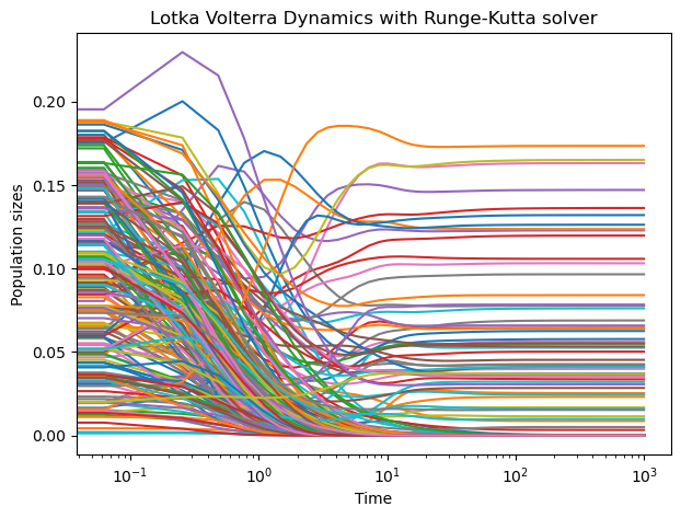

lvj = LotkaVolterraWithJacobian(N, random_state=0)
sol = solve_ivp(lvj.rhs, [0, 1000], n0, jac=lvj.jacobian, method="LSODA")
plt.figure(figsize=(7, 5))
plt.semilogx(sol.t, sol.y.T);
plt.xlabel("Time")
plt.ylabel("Population sizes")
plt.title("Lotka Volterra Dynamics with Implicit solver")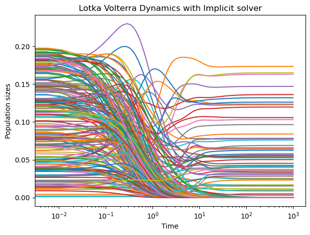

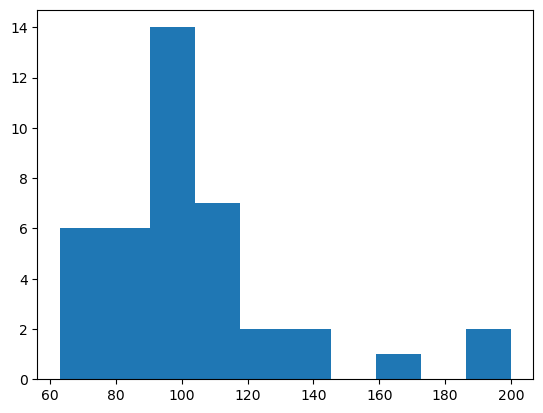
## Sample many random ecosystems, and study their asymptotic dynamics

num_survivors = list()
for seed in range(40):
    lvj = LotkaVolterraWithJacobian(N, random_state=seed)
    n0 = np.random.uniform(size=(N,))

    # sol = solve_ivp(lvj.rhs, [0, 1000], n0)
    sol = solve_ivp(lvj.rhs, [0, 1000], n0, jac=lvj.jacobian, method="Radau")

    num_survive = np.sum(sol.y[:, -1] > 1e-24)
    num_survivors.append(num_survive)

plt.hist(num_survivors)
print(f"The mean number of survivors is {np.mean(num_survivors)}")
print(f"The standard deviation of the number of survivors is {np.std(num_survivors)}")

The mean number of survivors is 103.8
The standard deviation of the number of survivors is 29.409352254002467

Additional information¶

The predator-prey dynamics of lynxes and hares in the Canadian wilderness turn out to have slightly more complex dynamics than the simple two-species model we have considered here. Modern analysis using tools for estimating the dimensionality of time series data suggest that multiple other species are coupled into the dynamics of the lynx and hare populations, such as Great-horned owls and coyotes.

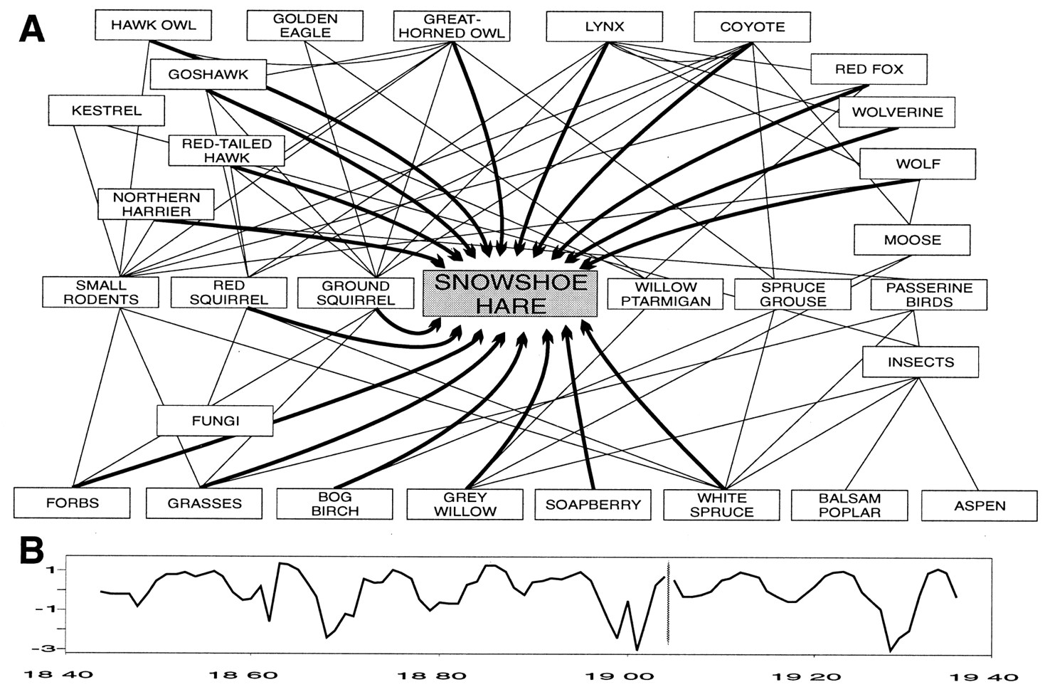
Image from Stenseth, et al. 1997 (PNAS)

References¶

Serván, C. A., Capitán, J. A., Grilli, J., Morrison, K. E., & Allesina, S. (2018). Coexistence of many species in random ecosystems. Nature Ecology & Evolution, 2(8), 1237–1242. 10.1038/s41559-018-0603-6
Stenseth, N. Chr., Falck, W., Bjørnstad, O. N., & Krebs, C. J. (1997). Population regulation in snowshoe hare and Canadian lynx: Asymmetric food web configurations between hare and lynx. Proceedings of the National Academy of Sciences, 94(10), 5147–5152. 10.1073/pnas.94.10.5147

Homework

The Power Method, Unsupervised Learning, and Principal Components Analysis

Homework

Partial differential equations, reaction-diffusion, and phase separation