
Preamble: Run the cells below to import the necessary Python packages
import numpy as np

# Import local plotting functions and in-notebook display functions
import matplotlib.pyplot as plt
from IPython.display import display, clear_output, Image

%matplotlib inline
Partial differential equations
We can think of partial differential equations (PDEs) as an infinite set of ordinary differential equations (ODEs). In numerical methods, we split up this set into a finite set of ODEs, usually by “meshing” the domain into a finite set of points.
There are several types of PDEs, elliptical, hyperbolic, and parabolic.
| Type | Equation | Example |
|---|---|---|
| Elliptical | Laplace’s equation | |
| Hyperbolic | Wave equation | |
| Parabolic | Heat equation |
where and in the table.
We will start by focusing on elliptical and parabolic PDEs.
Diffusion in free space
Suppose we have a quantity that is diffusing in free space. The diffusion equation states that the rate of change of is proportional to the Laplacian of
where is the diffusion constant or diffusivity, which determines how quickly the quantity diffuses. While many analytical solutions exist for the diffusion equation, numerical solutions are particularly valuable for more complicated geometries.
Laplace’s equation
With the diffusion equation, we are usually particularly interested in the steady-state solution, after the system has reached equilibrium. In this case, the time derivative is zero, and the diffusion equation becomes Laplace’s equation
The steady-state solution to Laplace’s equation gives the equilibrium distribution of in space. This is strongly influenced by the boundary conditions for the system. If the boundary conditions are trivial, as in the Dirichlet boundary conditions everywhere on the boundary, then the solution is trivial . However, if the boundary conditions are non-trivial, then the solution can be quite complex
Boundary value problems
Given some specificiation of the value of , , or some combination of these on the boundary of the system, we can solve for the steady-state solution to Laplace’s equation. This is called a boundary value problem.
We will focus initially on the case of Dirichlet boundary conditions, where the values of are specified to equal fixed values on the boundary of the system. Another option would be Neumann boundary conditions, where (the flux of scalar into the system) is instead specified on the boundary of the system.
Relaxation Methods for solving Laplace’s equation
The interior region in a boundary value problem contains no sources or sinks for the diffusing quantity . This means that the value of at some point in the interior of domain is equal to the average value of on the bounday of any enclosing ring via the mean value theorem,
where is the boundary of a disk of radius containing . This property gives rise to the smoothness of solutions to the Laplace equation.
Relaxation method
While the mean value property holds globally for any ring around any point in the domain, we can use it to derive an integration scheme in the limit where the enclosing ring corresponds to a discrete spatial mesh of the domain. If discrete spatial points in a 2D domain are indexed by and , then the mean value property can be written as
where is the value of at the point in the mesh. This is a self-consistent equation for , since the right-hand side is a function of and its nearest neighbors. We can solve this equation iteratively, starting with some initial guess for , and then updating the value of at each point in the mesh until the solution converges.
Notice that we are using the Von Neumann neighborhood, in contrast to the Moore neighborhood used in the Ising model and in many convolutional models.
class LaplaceEquation:
    """
    Class to solve the Laplace equation in 2D using the Jacobi method.

    Attributes:
        initial_lattice (np.ndarray): Initial lattice with boundary conditions
        max_iterations (int): Maximum number of iterations
        tolerance (float): Tolerance for convergence
        store_history (bool): Whether to store the history of the grid at each iteration

    Methods:
        solve: Solve the Laplace equation
        update_grid: Update the grid site-by-site

    """

    def __init__(self, initial_lattice, max_iterations=10000, tolerance=1e-4, store_history=False):
        self.initial_lattice = initial_lattice
        self.n, self.m = initial_lattice.shape
        self.max_iterations = max_iterations
        self.tolerance = tolerance
        self.store_history = store_history

    def solve(self):

        ## Initialize grid with zeros
        grid = np.copy(self.initial_lattice)

        if self.store_history:
            self.history = [grid.copy()]

        ## Iterate until convergence
        for iteration in range(self.max_iterations):
            # Copy current grid
            grid_old = np.copy(grid)

            # The actual update and physical simulation goes here
            grid = self.update_grid(grid)
            #y = self.update(t, y)

            ## Store history
            if self.store_history:
                self.history.append(grid.copy())

            ## Check for convergence
            if np.linalg.norm(grid - grid_old) < self.tolerance:
                print('Converged after {} iterations.'.format(iteration))
                break

        return grid

    def update_grid(self, grid):

        # ## Update grid site-by-site
        # for i in range(1, self.n - 1):
        #     for j in range(1, self.m - 1):
        #         grid[i, j] = 0.25 * (grid[i - 1, j] + grid[i + 1, j] + grid[i, j - 1] + grid[i, j + 1])

         ## Vectorized implementation of the above loop
        grid[1:-1, 1:-1] = 0.25 * (grid[:-2, 1:-1] + grid[2:, 1:-1] + grid[1:-1, 0:-2] + grid[1:-1, 2:])
        # grid[1:-1, 1:-1] = 0.25 * (grid[0:-2, 1:-1] + grid[2:, 1:-1] + grid[1:-1, 0:-2] + grid[1:-1, 2:])

        return grid
# Define initial lattice and complex boundary conditions
n_x = 100
# n_x = 10
# n_x = 4
initial_lattice = np.zeros((n_x, n_x))
# initial_lattice = np.random.uniform(0, 1, size=(n_x, n_x))
initial_lattice[0, :] = np.sin(np.linspace(0, 2 * np.pi, n_x))
initial_lattice[-1, :] = np.sin(np.linspace(0, 2 * np.pi * 5, n_x))
initial_lattice[:, 0] = np.sin(np.linspace(0, 2 * np.pi * 3, n_x))
initial_lattice[:, -1] = np.sin(np.linspace(0, 2 * np.pi / 3, n_x))

## Plot North, South, East, and West boundary conditions
plt.figure(figsize=(10, 10))
plt.subplot(221)
plt.plot(initial_lattice[0, 1:-1])
plt.xlabel('x'); plt.ylabel('V')
plt.title('North')
plt.subplot(222)
plt.plot(initial_lattice[-1, 1:-1])
plt.xlabel('x'); plt.ylabel('V')
plt.title('South')
plt.subplot(223)
plt.plot(initial_lattice[:, 0])
plt.xlabel('y'); plt.ylabel('V')
plt.title('West')
plt.subplot(224)
plt.plot(initial_lattice[:, -1])
plt.xlabel('y'); plt.ylabel('V')
plt.title('East')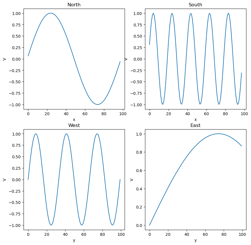
initial_latticearray([[ 0.00000000e+00, 6.34239197e-02, 1.26592454e-01, ...,
-1.26592454e-01, -6.34239197e-02, 0.00000000e+00],
[ 1.89251244e-01, -3.48313436e-01, -1.59011702e+00, ...,
2.15448227e+00, 6.81686265e-02, 2.11539281e-02],
[ 3.71662456e-01, -3.79450346e-02, 6.98809572e-01, ...,
-4.22074091e-01, -5.22006247e-01, 4.22983890e-02],
...,
[-3.71662456e-01, -1.13573146e+00, 1.43299057e+00, ...,
4.35043561e-01, -7.06004728e-01, 8.86399525e-01],
[-1.89251244e-01, -2.80691958e-01, -3.40423010e-01, ...,
5.09561004e-01, -9.87557567e-01, 8.76408578e-01],
[-7.34788079e-16, 3.12033446e-01, 5.92907929e-01, ...,
-5.92907929e-01, -3.12033446e-01, 8.66025404e-01]],
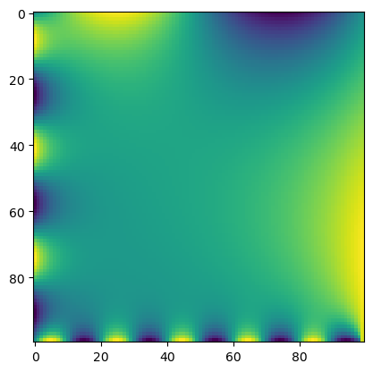
shape=(100, 100))# Solve Laplace equation
model = LaplaceEquation(initial_lattice, max_iterations=10000, store_history=True)
grid = model.solve()
# # Plot grid
plt.imshow(grid, interpolation='nearest')Converged after 8670 iterations.
## Make an interactive video
from ipywidgets import interact, interactive, fixed, interact_manual, Layout
from IPython.display import display
import ipywidgets as widgets


def plotter(i):
    plt.figure(figsize=(6, 6))
    plt.imshow(model.history[i], interpolation='nearest')
    plt.axis('off')
    plt.show()

interact(
    plotter,
    i=widgets.IntSlider(0, 0, len(model.history) - 1, 1)
)<function __main__.plotter(i)>Does this match our intuition?
The diffusion term appears to smooth out fluctuations in the field over time, This is a consequence of the intermediate value theorem for harmonic functions, which states that extrema of harmonic functions are always on boundaries, therefore no interior extrema are possible. Note that our implementation of relaxation is a synchronous update (all sites are updated at the same time), similar to the synchronous update we previously used for cellular automata.
Another approach: Convolutions
The inner loop of our solution method consists of visiting each point in the mesh, and then updating its value based on the average of its neighbors. This is a very simple operation, but it is repeated many times. This update rule is extremely similar to the Game of Life, and other cellular automata that we have seen previously.
Mathematically, we can think of the Laplace equation as a convolution of the potential with a kernel that is a function of the distance between the points. A convolution has the form:
where and are functions, and is the convolution operator. In discrete form, this becomes:
where and are now arrays of values, and is the discrete convolution operator. The convolutional kernel is the function , and it usually only exists on a compact interval. For the Laplace equation, the kernel in continuous time is a Gaussian, and in discrete time is a function that returns only the values of North, South, East, and West neighbors.
We can implement this in Python using the scipy.signal.convolve2d function.
from scipy.signal import convolve2d

class LaplaceEquationConvolution(LaplaceEquation):

    def __init__(self, *args, **kwargs):
        super().__init__(*args, **kwargs)

    def update_grid(self, grid):

        ## Define convolution kernel (von Neumann neighborhood)
        kernel = 0.25 * np.array([[0, 1, 0], [1, 0, 1], [0, 1, 0]])

        ## Convolve grid with kernel. Note how we handle the boundary conditions.
        grid[1:-1, 1:-1] = convolve2d(grid, kernel, mode='same')[1:-1, 1:-1]

        return grid
Let’s test out this new approach, to see how it compares to our previous implementation.
## Solve Laplace equation
model = LaplaceEquationConvolution(initial_lattice, max_iterations=1000, store_history=True)

grid = model.solve()

# Plot grid
plt.imshow(grid, interpolation='nearest')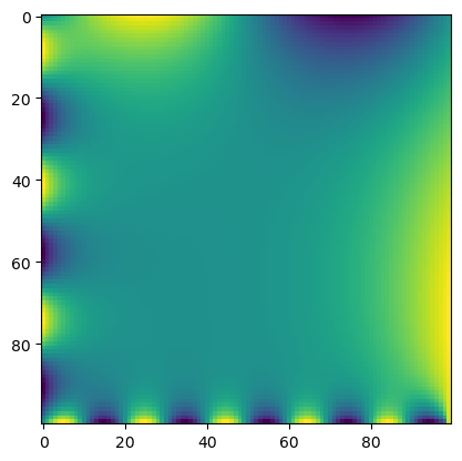
We can also plot the evolution of the field at a single lattice site over time.
plt.plot([item[10, 10] for item in model.history])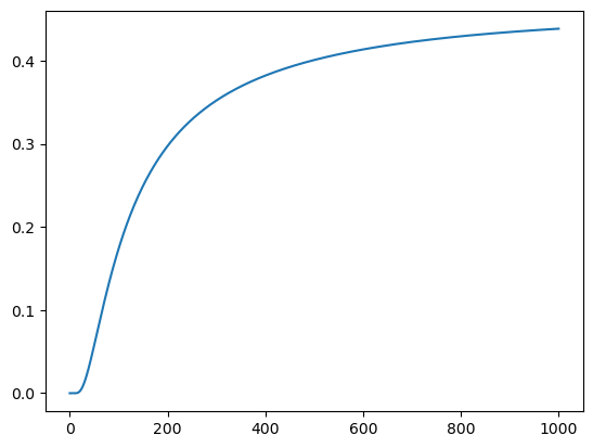
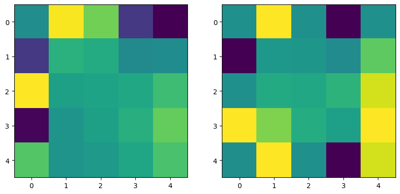
How does the accuracy depend on the mesh size?
The critical assumption in the relaxation method is that the mean value property holds for the discrete mesh. This degrades as the mesh size increases, because the mesh values no longer approximate a continuous contour. Below, we perform two simulations, one with a fine mesh and one with a coarse mesh. We then downsample the results of the fine mesh to the coarse mesh, in order to see what the “ground truth” should be for the coarse mesh
downsample_factor = 20

n_x = 100
initial_lattice = np.zeros((n_x, n_x))
initial_lattice[0, :] = np.sin(np.linspace(0, 2 * np.pi, n_x))
initial_lattice[-1, :] = np.sin(np.linspace(0, 2 * np.pi * 5, n_x))
initial_lattice[:, 0] = np.sin(np.linspace(0, 2 * np.pi * 3, n_x))
initial_lattice[:, -1] = np.sin(np.linspace(0, 2 * np.pi / 3, n_x))
model = LaplaceEquation(initial_lattice, max_iterations=10000, store_history=True)
grid1 = model.solve()


n_x = n_x // downsample_factor
initial_lattice = np.zeros((n_x, n_x))
initial_lattice[0, :] = np.sin(np.linspace(0, 2 * np.pi, n_x))
initial_lattice[-1, :] = np.sin(np.linspace(0, 2 * np.pi * 5, n_x))
initial_lattice[:, 0] = np.sin(np.linspace(0, 2 * np.pi * 3, n_x))
initial_lattice[:, -1] = np.sin(np.linspace(0, 2 * np.pi / 3, n_x))
model = LaplaceEquation(initial_lattice, max_iterations=10000, store_history=True)
grid2 = model.solve()


## Plot side-by-side
plt.figure(figsize=(10, 5))
plt.subplot(121)
plt.imshow(grid1[::downsample_factor, ::downsample_factor], interpolation='nearest')
plt.subplot(122)
plt.imshow(grid2, interpolation='nearest')
Converged after 5023 iterations.
Converged after 12 iterations.
Remember the convolution theorem?
where is the Fourier transform. This is a very useful result, because it allows us to convolve functions in the frequency domain, which is much faster than convolving in the time domain.
This is a clue that the Fourier transform is a useful tool for solving PDEs.
Intuition: sines and cosines are the eigenfunctions of translation operators
Links to cellular automata
Our convolutional implementation of the Laplace equation is very similar to the Game of Life implementation that we saw earlier in the course. In general, many cellular automata have integral update structure, where each site is updated based on the values of its neighbors. However, we have also seen examples of cellular automata with differential update structure, where a set of neighbors is updated based on their difference from the center site. The sandpile model is an example of this.
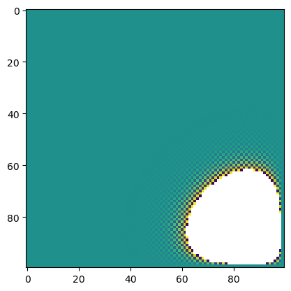
Solving Laplace’s equation with finite-differences
With the Laplace equation, we were able to use our domain knowledge to devise a relaxation solution scheme that approximates the path integral around a mesh cell.
In general, we can’t usually do this for other PDEs. Instead, we must use a more general method to solve the differential equation. The simplest method is to use a finite-difference method, which is a method of approximating the derivative of a function by using the values of the function at two or more points.
Suppose that we want to solve the heat equation in a 2D domain, , where the initial condition is , and the boundary conditions are for and . The heat equation is:
where is the thermal diffusivity. We can solve this equation by discretizing in time, and then using the finite difference method to discretize in space. The resulting equation is:
where is the value of at the point at time . We can rearrange this equation to solve for :
We can use the same approach as before, and use a loop to update the values of at each time step.
class LaplaceFiniteDifference:
    """
    A class to solve the Laplace equation using the finite difference method.

    Attributes:
        initial_lattice : np.ndarray
            The initial state of the lattice/grid.
        diffusivity : float, optional
            The diffusivity constant (default is 1.0).
        dt : float, optional
            The time step size (default is 1e-3).
        L : float, optional
            The length of the domain (default is 1.0).
        max_iterations : int, optional
            The maximum number of iterations (default is 10000).
        tolerance : float, optional
            The convergence tolerance (default is 1e-4).
        store_history : bool, optional
            Whether to store the history of the grid states (default is False).

    Methods:
        solve():
            Solves the Laplace equation until convergence or maximum iterations.
        update_grid(grid):
            Updates the grid using the finite difference method.
    """

    def __init__(self, initial_lattice, diffusivity=1.0, dt=1e-3, L=1.0,
                 max_iterations=20000, tolerance=1e-5, store_history=False):

        self.initial_lattice = initial_lattice
        self.max_iterations = max_iterations
        self.tolerance = tolerance

        self.store_history = store_history
        self.diffusivity = diffusivity
        self.dt = dt
        self.dx = L / (initial_lattice.shape[0] - 1)

    def solve(self):

        ## Initialize grid
        grid = self.initial_lattice.copy()

        ## Initialize history
        if self.store_history:
            self.history = [grid.copy()]

        ## Initialize iteration counter
        iteration = 0

        ## Initialize error
        error = np.inf

        ## Iterate until convergence
        while iteration < self.max_iterations and error > self.tolerance:

            ## Update grid
            grid = self.update_grid(grid)

            ## Update iteration counter
            iteration += 1

            ## Update error
            error = np.max(np.abs(grid - self.history[-1]))
            if error < self.tolerance:
                print(f'Converged after {iteration} iterations.')
                break
            ## Update history
            if self.store_history:
                self.history.append(grid.copy())

        return grid

    def update_grid(self, grid):
        ## Update grid using finite difference method

        k1 = grid[1:-1, 1:-1]
        k2 = grid[1:-1, 2:]
        k3 = grid[1:-1, :-2]
        k4 = grid[2:, 1:-1]
        k5 = grid[:-2, 1:-1]

        grid[1:-1, 1:-1] = grid[1:-1, 1:-1] + self.dt * self.diffusivity * (k2 + k3 + k4 + k5 - 4 * k1) / self.dx**2
        # grid[1:-1, 1:-1] = grid[1:-1, 1:-1] + self.dt * self.diffusivity * (k2 + k3 + k4 + k5 - 4 * k1) / self.dx**2

        return grid


# Define initial lattice and complex boundary conditions
n_x = 100
initial_lattice = np.zeros((n_x, n_x))
initial_lattice[0, :] = np.sin(np.linspace(0, 2 * np.pi, n_x))
initial_lattice[-1, :] = np.sin(np.linspace(0, 2 * np.pi * 5, n_x))
initial_lattice[:, 0] = np.sin(np.linspace(0, 2 * np.pi * 3, n_x))
initial_lattice[:, -1] = np.sin(np.linspace(0, 2 * np.pi / 3, n_x))

# from scipy.signal import convolve2d

## Solve Laplace equation
# model = LaplaceFiniteDifference(initial_lattice, dt=1e-3, max_iterations=10000, store_history=True)
# model = LaplaceFiniteDifference(initial_lattice, dt=1e-4, max_iterations=10000, store_history=True)
model = LaplaceFiniteDifference(initial_lattice, dt=6e-5, max_iterations=20000, store_history=True)

grid = model.solve()

# Plot grid
plt.imshow(model.history[-1], interpolation='nearest')
/var/folders/79/zct6q7kx2yl6b1ryp2rsfbtc0000gr/T/ipykernel_59645/4092704738.py:84: RuntimeWarning: overflow encountered in add
  grid[1:-1, 1:-1] = grid[1:-1, 1:-1] + self.dt * self.diffusivity * (k2 + k3 + k4 + k5 - 4 * k1) / self.dx**2
/var/folders/79/zct6q7kx2yl6b1ryp2rsfbtc0000gr/T/ipykernel_59645/4092704738.py:84: RuntimeWarning: overflow encountered in multiply
  grid[1:-1, 1:-1] = grid[1:-1, 1:-1] + self.dt * self.diffusivity * (k2 + k3 + k4 + k5 - 4 * k1) / self.dx**2
/var/folders/79/zct6q7kx2yl6b1ryp2rsfbtc0000gr/T/ipykernel_59645/4092704738.py:84: RuntimeWarning: overflow encountered in subtract
  grid[1:-1, 1:-1] = grid[1:-1, 1:-1] + self.dt * self.diffusivity * (k2 + k3 + k4 + k5 - 4 * k1) / self.dx**2
/var/folders/79/zct6q7kx2yl6b1ryp2rsfbtc0000gr/T/ipykernel_59645/4092704738.py:84: RuntimeWarning: invalid value encountered in add
  grid[1:-1, 1:-1] = grid[1:-1, 1:-1] + self.dt * self.diffusivity * (k2 + k3 + k4 + k5 - 4 * k1) / self.dx**2
1/(model.diffusivity * 2 / model.dx**2)5.101520253035405e-05plt.plot([item[10, 10] for item in model.history])
plt.xlabel('Iteration')
plt.ylabel('Scalar field at middle pixel')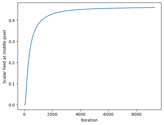
## Make an interactive video
from ipywidgets import interact, interactive, fixed, interact_manual, Layout
from IPython.display import display
import ipywidgets as widgets


def plotter(i):
    plt.figure(figsize=(6, 6))
    plt.imshow(model.history[i], interpolation='nearest')
    plt.axis('off')
    plt.show()

interact(
    plotter,
    i=widgets.IntSlider(0, 0, len(model.history) - 1, 1)
)<function __main__.plotter(i)>Questions
Try modifying the space and time steps. What happens to the solution?
How would you expect the solution to change if the domain was a disk? Or a ring?
Stability of finite-difference schemes for the diffusion equation
The 1D Laplacian is a matrix
To understand the origin of instability, let’s write down the 1D discretized diffusion equation.
We can write this as a discrete-time update equation in matrix form:
where is a vector of the values of at each point in the mesh, and is the 1D Laplacian matrix.
The 1D Laplacian is a matrix, and we can use matrix algebra to represent some operators. If we have points in our discretized mesh of , then 1D Laplacian is given by and matrix:
In 2D we are not so lucky. We have to use convolutions, or flatten the lattice into a vector of length . But the linear operator can still be defined in the same way.
Boundary conditions
For our examples so far, we’ve specified the boundary conditions as for all , where denotes our solution domain (square, disk, etc).
Our cases so far have been Dirichlet boundary conditions, where we specify the value of at the boundary.
We can also have Neumann boundary conditions, where we specify the value of the derivative of at the boundary. For example, we could specify for all , where is a unit vector normal to the boundary. This type of boundary condition specifies a fixed flux of the scalar field through the boundary.
We can also have mixed or Robin boundary conditions, where we specify a combination of Dirichlet and Neumann boundary conditions. for all .
1D Laplacian with various boundary conditions
The 1D Laplacian with Dirichlet boundary conditions has the form
The 1D Laplacian with Neumann (reflection) boundary conditions has the form
The 1D Laplacian with periodic boundary conditions has the form
Stability of finite difference schemes
The 1D discretized diffusion equation is given by
we can group terms on the right-hand side to get
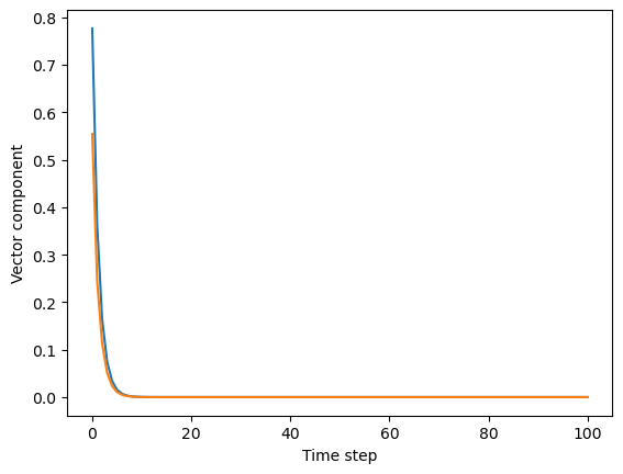
Recall that a linear dynamical system has the form
where is a matrix. We can think of this as a map from .
Depending on whether , , or , the system will be stable, marginally stable, or unstable.
## Sample a random 2 x 2 symmetric matrix
a = 0.3 * np.random.random((2, 2))
# a = np.random.random((2, 2))
a += a.T
print("Eigenvalues of symmetric transition matrix: ", np.linalg.eigvals(a))

## Simulate dynamics starting from a random initial 2D vector
all_u = [np.random.random(2)]
for _ in range(100):
    all_u.append(a @ all_u[-1])
all_u = np.array(all_u)

plt.figure()
plt.plot(all_u[:, 0])
plt.plot(all_u[:, 1])
plt.ylabel("Vector component")
plt.xlabel("Time step")
Eigenvalues of symmetric transition matrix: [ 0.45685674 -0.1443018 ]
Implementing a finite difference scheme for the 1D diffusion equation
In one dimension, the diffusion equation is given by
We can approximate this equation using first-order finite differences in space and time
We use the index to denote different lattice points in space, and to denote different time steps. We rearrange terms to write this equation as a matrix equation that updates at each time step
Notice that we can write the right-hand side of this differential equation as a constant matrix acting on the vector
where is a tridiagonal matrix with -2 on the diagonal, and 1 on the off-diagonals. In general, we can always write linear partial differential equations as linear matrix equations in discrete time.
def laplacian(n, dx=1.0):
"""
Create a one-dimensional discrete Laplacian operator with periodic boundary conditions.
Args:
n (int): The number of grid points.
dx (float): The grid spacing.
Returns:
ndarray: The Laplacian operator in one dimension.
"""
op = np.zeros((n, n))
# set diag to -2
np.fill_diagonal(op, -2)
# set off-diag to 1
np.fill_diagonal(op[:, 1:], 1)
np.fill_diagonal(op[1:, :], 1)
# set periodic boundary conditions
op[0, -1] = 1
op[-1, 0] = 1
return op / dx**2
class DiscretizedPDE:
"""
A base class for discretized PDEs in one dimension.
Parameters
n (int): The number of grid points in one dimension
dx (float): The grid spacing
dt (float): The time step
store_history (bool): Whether to store the history of the solution
random_state (int): The random seed
"""
def __init__(self, n, dx=1.0, dt=1.0, store_history=True, random_state=0, verbose=False):
self.n = n
self.dt = dt
self.dx = dx
self.store_history = store_history
self.random_state = random_state
self.verbose = verbose
def rhs(self, u):
raise NotImplementedError
def solve(self, u0, nt):
u = u0
if self.store_history:
self.history = [u0.copy()]
for i in range(nt):
u += self.rhs(u) * self.dt
if self.store_history:
self.history.append(u.copy())
return u
class DiffusionEquation(DiscretizedPDE):
"""
A class for discretized diffusion equations in one dimension.
"""
def __init__(self, D=1.0, **kwargs):
super().__init__(**kwargs)
self.D = D
self.lap = laplacian(self.n, self.dx)
if self.verbose:
## print the eigenvalues of the iteration operator
print("Max norm eigenvalues of update operator: ",
np.max(
np.abs(
np.linalg.eigvals(np.eye(self.n) + self.D * self.dt * self.lap
)
)
)
)
def rhs(self, u):
return self.D * self.lap @ u
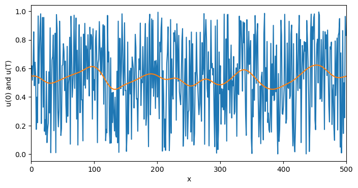
eq = DiffusionEquation(n=500, dx=1.0, dt=0.08, D=1.0, store_history=True, verbose=True)
# eq = DiffusionEquation(n=500, dx=1.0, dt=1.0, D=1.0, store_history=True, verbose=True)
# Initial condition
u0 = np.random.random(500).copy()
# Solve the equation
u = eq.solve(u0, 1000)
plt.figure(figsize=(8, 4))
plt.plot(eq.history[0])
plt.plot(eq.history[-1])
plt.xlim(0, len(u0))
plt.xlabel("x")
plt.ylabel("u(0) and u(T)")
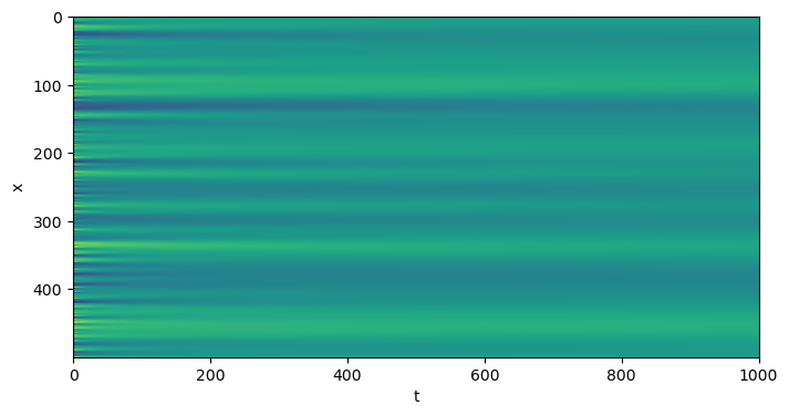
plt.figure(figsize=(8, 4))
plt.imshow(np.array(eq.history).T, aspect='auto')
plt.xlabel("t")
plt.ylabel("x")
Max norm eigenvalues of update operator: 0.9999999999999977
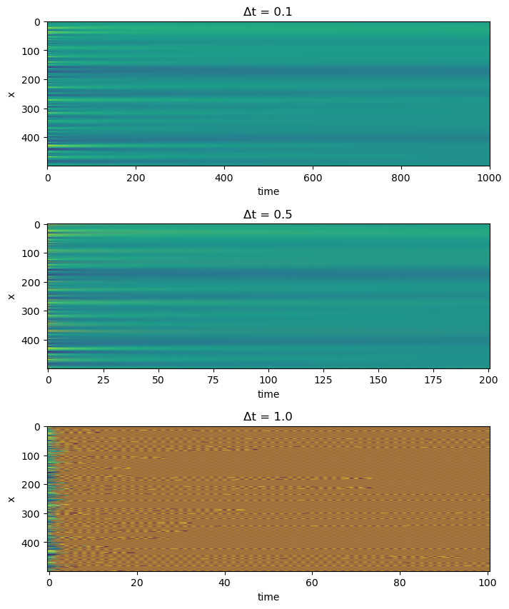
Can we perform fewer operations?
Suppose we want to do the numerical integration a lot faster. One option might be to increase and . But is there a limit to how far we can go? Let’s do a simple experiment to find out.
# Initial condition
u0 = np.random.random(500)

# make three subplots
fig, axes = plt.subplots(3, 1, figsize=(8, 10))
plt.subplots_adjust(wspace=0.0, hspace=0.4)

eq = DiffusionEquation(n=500, dx=1.0, dt=0.1, D=1.0, store_history=True, verbose=True)
u = eq.solve(u0.copy(), 1000)

# make figure subplot
plt.subplot(3, 1, 1)
plt.imshow(np.array(eq.history).T, aspect='auto', vmin=0, vmax=1)
plt.xlabel("time")
plt.ylabel("x")
plt.title("Δt = 0.1")

eq = DiffusionEquation(n=500, dx=1.0, dt=0.5, D=1.0, store_history=True, verbose=True)
u = eq.solve(u0.copy(), 200)
plt.subplot(3, 1, 2)
plt.imshow(np.array(eq.history).T, aspect='auto', vmin=0, vmax=1)
plt.xlabel("time")
plt.ylabel("x")
plt.title("Δt = 0.5")

eq = DiffusionEquation(n=500, dx=1.0, dt=1.0, D=1.0, store_history=True, verbose=True)
u = eq.solve(u0.copy(), 100)
plt.subplot(3, 1, 3)
plt.imshow(np.array(eq.history).T, aspect='auto', vmin=0, vmax=1)
plt.xlabel("time")
plt.ylabel("x")
plt.title("Δt = 1.0")
Max norm eigenvalues of update operator:  0.9999999999999993
Max norm eigenvalues of update operator:  1.0
Max norm eigenvalues of update operator:  3.0000000000000164
We now repeat this experiment for many different values of the timestep
dt_vals = np.logspace(-2, 0, 200)
max_field = []
for dt_val in dt_vals:
    eq = DiffusionEquation(n=500, dx=1.0, dt=dt_val, D=1.0, store_history=True)
    u = eq.solve(u0.copy(), 400)
    max_field.append(np.max(np.abs(u)))

plt.figure()
plt.loglog(dt_vals, max_field, '.')
plt.xlabel("Δt")
plt.ylabel("Max field value")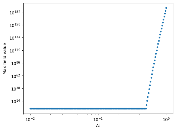
We suspect that this instability arises due to the matrix that we are iterating changing from having a converging behavior to a diverging behavior, as we saw above. Because the growth factor is a function of the largest eigenvalues of the matrix (as we saw in the power method), we can show this instability analytically.
Recall that our discrete time, discrete-space diffusion equation is
Due to the periodic boundary conditions, can be shown that the eigenvalues of are
where is the number of lattice points and . We are particularly interested in the maximum eigenvalue, which determines the growth factor of the system after many iterations.
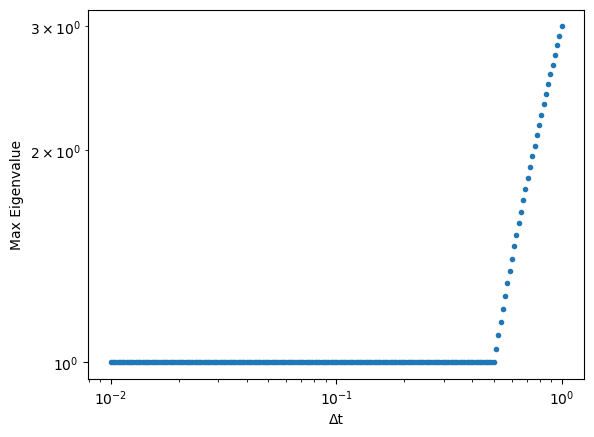
We can compute the spectrum analytically for the choices of , , and that we used in the simulation above. We can then plot the expected maximum eigenvalue as a function of .
def eigenvalues_diffusion(n, dx=1.0, dt=1.0, D=1.0):
"""
Compute the eigenvalues of the diffusion equation in one dimension.
Args:
n (int): The number of grid points.
dx (float): The grid spacing.
dt (float): The time step.
D (float): The diffusion coefficient.
Returns:
ndarray: The eigenvalues of the diffusion equation.
"""
nvals = np.arange(n)
return 1 - (D * dt / dx**2) * (2 * np.cos(np.pi * nvals / n) + 2)
# plt.plot(eigenvalues_diffusion(500, dt=0.1, D=1.0))
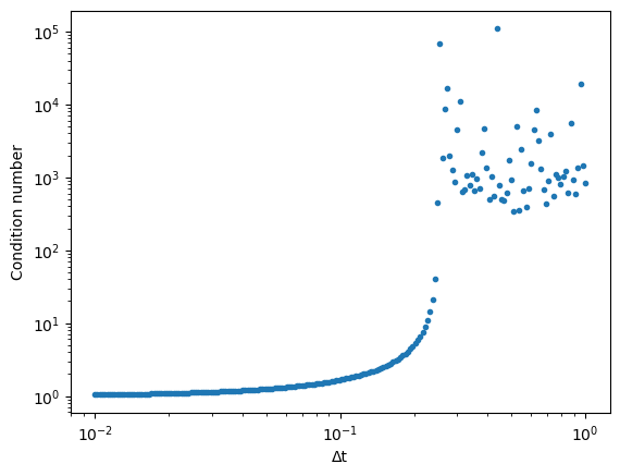
max_eig, min_eig = [], []
all_conds = []
p2 = []
for dt_val in dt_vals:
eigs_diff = eigenvalues_diffusion(500, dx=1.0, dt=dt_val, D=1.0)
max_eig.append(np.max(np.abs(eigs_diff)))
min_eig.append(np.min(np.abs(eigs_diff)))
cond = np.max(np.abs(eigs_diff)) / np.min(np.abs(eigs_diff))
all_conds.append(cond)
# plt.plot(eigs_diff)
## We could also compute the condition number of the propagation matrix directly
## But this is more computationally expensive
# eq = DiffusionEquation(n=500, dx=1.0, dt=dt_val, D=1.0)
# prop = np.identity(500) + (eq.D * eq.dt / eq.dx**2) * eq.lap
# cond = np.linalg.cond(prop)
# all_conds.append(cond)
plt.figure()
plt.loglog(dt_vals, max_eig, '.')
plt.xlabel("Δt")
plt.ylabel("Max Eigenvalue")
plt.figure()
plt.loglog(dt_vals, all_conds, '.')
plt.xlabel("Δt")
plt.ylabel("Condition number")
# n=500, dx=1.0, dt=dt_val, D=1.0,
von Neumann stability condition
We can see that the abrupt divergence in the dynamics of the simulation arises from the largest-norm eigenvalue rapidly increasing as we increase . This abrupt change suggests that an abrupt change occurs in the underlying spectrum .
It turns out that we can trace this discontinuity to the discontinuous max function in . The value of that maximizes abruptly changes.
Because the cosine function changes monotonically on the interval , the only two options for the maximum occur at the endpoints of the interval . We see why this is the case by plotting the \abs{\lambda_n} as a function of for various values of .
dt_vals = np.logspace(-2, 0, 200)
def eigenvalues_diffusion(n, dx=1.0, dt=1.0, D=1.0):
    """
    Compute the eigenvalues of the diffusion equation in one dimension.

    Args:
        n (int): The number of grid points.
        dx (float): The grid spacing.
        dt (float): The time step.
        D (float): The diffusion coefficient.

    Returns:
        ndarray: The eigenvalues of the diffusion equation.
    """
    nvals = np.arange(n)
    return 1 - (D * dt / dx**2) * (2 * np.cos(np.pi * nvals / n) + 2)
for i, dt_val in enumerate(dt_vals[::20]):
eigs_diff = eigenvalues_diffusion(500, dx=1.0, dt=dt_val, D=1.0)
# plt.figure()
plt.plot(np.abs(eigs_diff), color=plt.cm.viridis(i / len(dt_vals[::20])))
plt.xlabel("Eigenvalue index")
plt.ylabel("Eigenvalue absolute value")
plt.legend(np.round(dt_vals[::20], 2), title="Δt")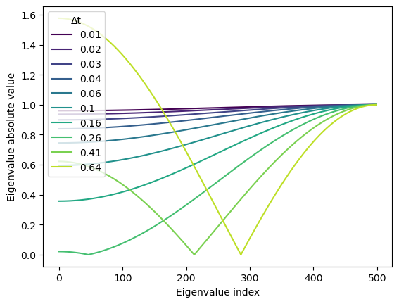
Thus, the maximum of the set of eigenvalues is at either end of the interval,
In the limit , we can simplify this expression,
The crossover point therefore corresponds to the condition
which, for our parameter values, corresponds to . This condition relating the diffusivity, timestep, and lattice discretization represents an example of von Neumann stability analysis for finite difference schemes.
Questions
Why did we call the
laplacianfunction in the__init__method of theDiffusionclass? Why not call it within therhsmethod?A common hyperbolic PDE is the wave equation:
where is the speed of the wave. Based on the stability conditions that we derived previously, what would you expect the linear stability condition for this equation to be?