Preamble: Run the cells below to import the necessary Python packages
Open this notebook in Google Colab: 
import numpy as np
from IPython.display import Image, display

import matplotlib.pyplot as plt
%matplotlib inline

%load_ext autoreload
%autoreload 2

import warnings
def fixed_aspect_ratio(ratio, ax=None, log=False, semilogy=False, semilogx=False):
    """
    Set a fixed aspect ratio on matplotlib plots regardless of the axis units
    """
    if not ax:
        ax = plt.gca()
    xvals, yvals = ax.axes.get_xlim(), ax.axes.get_ylim()
    xrange = np.abs(xvals[1] - xvals[0])
    yrange = np.abs(yvals[1] - yvals[0])
    if log:
        xrange = np.log10(xvals[1]) - np.log10(xvals[0])
        yrange = np.log10(yvals[1]) - np.log10(yvals[0])
    if semilogy:
        yrange = np.log10(yvals[1]) - np.log10(yvals[0])
    if semilogx:
        xrange = np.log10(xvals[1]) - np.log10(xvals[0])
    try:
        ax.set_aspect(ratio*(xrange/yrange), adjustable='box')
    except NotImplementedError:
        warnings.warn("Setting aspect ratio is experimental for 3D plots.")
        plt.gca().set_box_aspect((1, 1, ratio*(xrange/yrange)))
        #ax.set_box_aspect((ratio*(xrange/yrange), 1, 1))
The autoreload extension is already loaded. To reload it, use:
  %reload_ext autoreload
ODEs vs PDEs
While there are many strategies available for integrating an ODE, typically when we first encounter a new ODE to integrate, we can use built-in integration tools. The only exception is in the case of special types of differential equations (delay, integro-differential, etc.) PDEs, however, usually are not so straightforward. Each new PDE we encounter will have its own phenomenology, strategies, and limitations, and so we often have to analyze the structure of a PDE before picking a numerical strategy for solving it.
However, common PDE (Navier Stokes, Laplace, etc.) often have significant research behind them, and there may be external libraries that work in certain regimes, or which can help with meshing, etc. But even in very restricted regimes, the design of these tools is expensive and narrow. Using finite element tools like Ansys, COMSOL, etc. is a whole specialization in itself.
However, when figuring out how to tackle a PDE, it can be helpful to identify its broad properties. A particularly important designation is whether the PDE is elliptical, hyperbolic, and parabolic.
| Type | Equation | Example |
|---|---|---|
| Elliptic | Laplace’s equation | |
| Hyperbolic | Wave equation | |
| Parabolic | Heat equation |
where and in the table
We can see that the designation refers to the relationship between the order of time derivatives and space derivatives in the PDE. In general, in systems in which they are both the same order (such as first order in Burgers’ equation, or second order in the wave equation), the PDE will often exhibit waves and traveling solutions. In contrast when the derivatives are mixed, we tend to get spreading or coarsening solutions that distort as they change scales, as occurs in the diffusion equation.
In order to demonstrate the connections between simulating ODEs and simulating ODES, we will first implement ODE solver, similar to the ones used in previous lectures. We will structure this code with a base class BaseFixedStepIntegrator that will be inherited by specific solvers. This will allow us to easily switch between different solvers in the future.
## Define a fixed step integrator (solve_ivp uses adaptive step size)

class BaseFixedStepIntegrator:
    """
    A base class for fixed-step integration methods.
    """
    def __init__(self, dt=1e-3):
        self.dt = dt
        self.name = self.__class__.__name__

    def integrate(self, f, tspan, y0, t_eval=None):
        """
        Integrate the ODE y' = f(t, y) from t0 to tf using an integrator's update method
        """
        t0, tf = tspan

        # Create an array of time points to evaluate the solution
        t_sol = np.arange(t0, tf, self.dt)

        # Create an array to store the solution (pre-allocate)
        y = np.zeros((len(t_sol), len(y0)))

        # Set the initial condition
        y[0] = y0

        # Integrate the ODE
        for i in range(1, len(t_sol)):
             # this will be defined in the subclass:
            y[i] = self.update(f, t_sol[i - 1], y[i - 1])

        ## Resample the solution in y to match t_eval
        if t_eval:
            y_eval = np.interp(t_eval, t_sol, y)
            self.t, self.y = t_eval, y_eval
        else:
            self.t, self.y = t_sol, y
        return self

    def update(self, f, t, y):
        """
        Update the solution using the integrator's method
        """
        raise NotImplementedError("This method must be implemented in a subclass")


class RK4(BaseFixedStepIntegrator):
    """
    The 4th order Runge-Kutta integration scheme
    """
    def __init__(self, **kwargs):
        super().__init__(**kwargs)

    def update(self, f, t, y):
        k1 = f(t, y)
        k2 = f(t + self.dt / 2, y + self.dt * k1 / 2)
        k3 = f(t + self.dt / 2, y + self.dt * k2 / 2)
        k4 = f(t + self.dt, y + self.dt * k3)
        return y + self.dt * (k1 + 2 * k2 + 2 * k3 + k4) / 6
Just to test that everything is working as intended, we can try integrating a simple system, a pendulum.
## Test the integrator on a simple ODE

def pendulum(t, y):
    """
    The ODE describing a simple pendulum.
    """
    theta, omega = y
    return np.array([omega, -np.sin(theta)])

# Set the initial conditions
y0 = np.array([np.pi / 4, 0])

# Set the time span
tspan = [0, 10]

# Create the integrator\
integrator = RK4(dt=1e-2)

# Integrate the ODE
integrator.integrate(pendulum, tspan, y0)

# Plot the solution
plt.plot(integrator.t, integrator.y[:, 0])
plt.xlabel("Time")
plt.ylabel("Angle")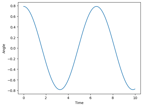
Determining boundary conditions
The boundary conditions are the conditions on the solution at of the PDE at edges of the domain, which includes both space and time for PDEs. In this sense, boundary conditions generalize the initial conditions we need to integrate ODEs. The boundary conditions are usually specified as functions of the integration variable(s) (like concentration or probability) as a function of the domain variables (e.g. starting or ending time, or position along an edge of the domain).
In a boundary value problem, we specify the boundary conditions as for all , where denotes our solution domain (square, disk, etc). These are known as Dirichlet boundary conditions, where we specify the value of at the boundary. We can also have Neumann boundary conditions, where we instead specify the value of the derivative of at the boundary. For example, we could specify for all , where is a unit vector normal to the boundary. This type of boundary condition specifies a fixed flux of the scalar field through the boundary. We can also have mixed or Robin boundary conditions, where we specify a combination of Dirichlet and Neumann boundary conditions. for all .
Burgers’ equation
Burgers’ equation is nonlinear partial differential equation describing the time evolution of the speed of a fluid in one dimension. This is a toy model of how steep waves form in shallow water in the ocean.
We will solve Burgers’ equation on a 1D domain of length , so . Burger’s equation is a one-dimensional partial differential equation. The integration variable is , and the domain variables are . Our boundary conditions and initial conditions will thus consist of the initial value of the field and the values of the velocity or acceleration at the edges of the domain . Because this equation has first order derivatives in both space and time, we consider it a hyperbolic equation. The solution of Burgers’ equation tend to evolve towards shocks, which are sharp discontinuities in the velocity.
Semi-discretization: The Method of lines
In a semi-discrete method, we explicitly discretize the spatial domain using finite differences, spectral projection, or something else. We then solve the resulting set of coupled ODEs in continuous time using a built-in ODE solver. This solver might also discretize time (implicitly or explicitly); however, this is handled independently of how we choose to discretize space. Mathematically, we can think of discretizing space as splitting a continuous PDE into a large set of coupled ODEs. The initial field value becomes the initial conditions, and the boundary conditions become a condition on how the ODEs are coupled together. The number of coupled ODEs depends on how finely we discretize space.
We will solve semi-discretized PDEs is using a built-in ODE solver. We therefore separate meshing (dealing with the domain) from timestepping (evolving forward in time)
Finite difference operators
The finite difference operators on particular choice of spatial discretization scheme. Finite difference operators essentially split space into small pieces with size . They then approximate spatial derivatives in the PDE on these discrete block.
The central first-order finite difference operators in 1D has the form
The central second-order finite difference operators in 1D has the form
We can see that, as the mesh becomes finer , the quality of the approximation increases.
Semi-discretizing Burgers’ equation
Using the finite-different approximations to approximate the spatial derivatives, Burgers’ equation becomes
We have a hyperparameter to set, which is the number of spatial points that we use to discretize the domain. . After performing this discretization, the field variable becomes . We can therefore write Burgers’ equation as a multivariate ODE, taking advantage of the fact that corresponds to the next index into the vector
The index tracks the different mesh points on the spatial site.
Boundary conditions
What happens when we get to the last value of the array? We can’t look up if . We now need to define, physically, what happens at the edges of our domain.
Periodic boundary conditions are simple to implement, but are not usually well-motived physically. The involve setting the condition that , and that
Dirichlet boundary conditions describe many physical systems, but may be less stable numerically. The involve setting a fixed value, like , and
Neumann boundary conditions are also very physical, and here they lead to mirror boundary conditions, where the walls of the domain reflect oncoming shocks. Since these involve conditions on the first derivative of the field with respect to space, we have to set these in terms of finite differences: , which is equivalent to the reflection symmetry . The same goes for the other side of the domain,
class BurgersEquation:
    """A class implementing Burgers' equation

    Parameters
        x (np.ndarray): The coordinates of the domain points
        t (np.ndarray): The timepoints at which to calculate the solution
        u0 (np.ndarray): The initial value of the speed variable across space at t=0
        nu (float): The value of the viscousity, which damps out the shocks

    """

    def __init__(self, x, t, u0, nu=1e-2):
        self.x = x
        self.t = t
        self.u0 = u0
        self.nu = nu

        self.dx = x[1] - x[0]

    def _derivative(self, u):
        du = u.copy()

        # Vectorized central finite difference by shifting the array forwards/backwards
        du[1:-1] = (u[2:] - u[:-2]) / (2 * self.dx)
        # for i in range(len(self.x)):

        ## Periodic boundary conditions
        du[0] = (u[1] - u[-1]) / self.dx
        du[-1] = (u[0] - u[-2]) / self.dx

        ## clamped (Dirichlet) boundary conditions
        # du[0] = (u[1] - 0) / self.dx
        # du[-1] = (0 - u[-1]) / self.dx

        ## Reflection (Neumann) boundary conditions
        # du[0] = 0
        # du[-1] = 0

        return du

    def _laplacian(self, u):
        ddu = u.copy()

        # Vectorized second order central finite difference by shifting the array
        # forwards/backwards twice
        ddu[1:-1] = (u[2:] - 2 * u[1:-1] + u[:-2]) / self.dx**2

        # Periodic boundary conditions
        ddu[0] = (u[1] - 2 * u[0] + u[-1]) / self.dx**2
        ddu[-1] = (u[0] - 2 * u[-1] + u[-2]) / self.dx**2

        ## clamped (Dirichlet) boundary conditions
        # ddu[0] = (u[1] - 2 * u[0] + 0) / self.dx**2
        # ddu[-1] = (0 - 2 * u[0] + u[-1]) / self.dx**2

        ## Reflection (Neumann) boundary conditions
        # ddu[0] = (u[1] - 2 * u[0] + u[1]) / self.dx**2
        # ddu[-1] = (u[-2] - 2 * u[-1] + u[-2]) / self.dx**2

        return ddu

    def rhs(self, t, u):
        return self.nu * self._laplacian(u) - u * self._derivative(u)

    def __call__(self, *args, **kwargs):
        return self.rhs(*args, **kwargs)
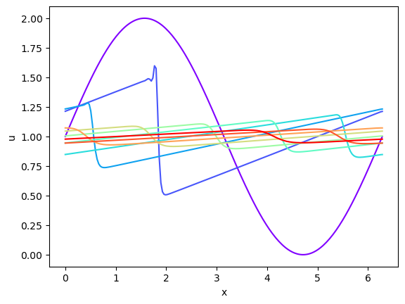
We can now try numerically solving this system with the method of lines, in order to explore the behavior of Burgers’ equation.
n_mesh = 200 # We set this hyperparameter, which decides the fineness of our mesh
# n_mesh = 30
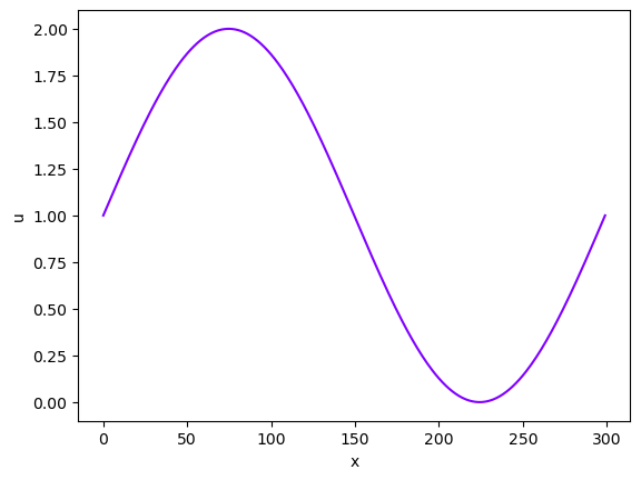
x = np.linspace(0, 2 * np.pi, n_mesh) # Initial x vector
t = np.linspace(0, 50, 800) #
# Initial field value at all x points need to pick an initial condition
# consistent with boundary conditions
u0 = 1 - np.cos(x)
eq = BurgersEquation(x, t, u0, nu=1e-2)
# plt.plot(x, u0)
# # from scipy.integrate import solve_ivp
# # sol = solve_ivp(eq, (t[0], t[-1]), u0, t_eval=t)
integrator = RK4(dt=1e-2)
sol = integrator.integrate(eq, (t[0], t[-1]), u0)
# plot with colormap for time
plt.figure()
colors = plt.cm.rainbow(np.linspace(0, 1, len(sol.y[::500])))
for i, sol0 in enumerate(sol.y[::500]):
plt.plot(x, sol0, color=colors[i])
plt.xlabel('x')
plt.ylabel('u')
plt.show()
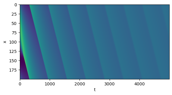
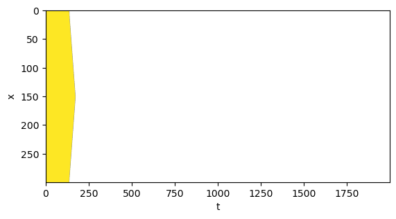
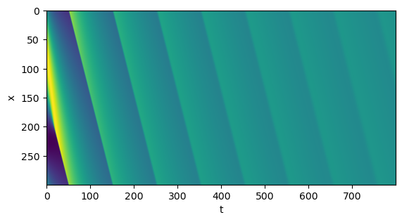
plt.figure()
plt.imshow(sol.y.T)
# plt.xlim([0, 900])
fixed_aspect_ratio(1/2)
plt.xlabel('t')
plt.ylabel('x')
# plt.colorbar(label='u(x, t)')
# plt.show()
plt.figure()
colors = plt.cm.rainbow(np.linspace(0, 1, len(sol.y[::500])))
for i, sol0 in enumerate(sol.y[::100][:10]):
    plt.plot(x, sol0, color=colors[i])
plt.xlabel('x')
plt.ylabel('u')
plt.show()

Explore the behavior of this PDE
Try playing with the parameters and to see how the solution evolves. What causes the shocks to live longer?
Try changing the initial condition to a Gaussian. What happens?
Try changing the boundary conditions to reflective (Neumann) or Dirichlet. What happens?
What happens as we change the timestep or the number of mesh points
The CFL condition for hyperbolic PDEs
The Courant–Friedrichs–Lewy (CFL) condition is a condition on mesh size and the time step that must be satisfied for the numerical solution of a hyperbolic PDE to be stable. Suppose that we have the wave equation in one dimension:
where determines the speed of travelling waves. A full discretization of this equation in space and time would be
The CFL condition determines the maximum value of that can be used for a given and
where the dimensionless Courant number is determined by our iteration scheme. The exact value of can be interpreted as the number of mesh cells that a particle of can traverse per integration time step (for an Euler time-stepping scheme and fixed mesh size, this is exact). Realistically, we want to stay a little bit below the CFL limit, because we don’t want to be right on the edge of instability. A typical “safety factor” would be .
Variants of the CFL condition also hold for other classes of PDEs. For example, the Neumann condition is a meshing condition for parabolic (diffusive) PDE: .
Applying the CFL condition to Burgers’ equation
While we typically use the CFL condition here for hyperbolic PDE (wave equations), in practice it’s a good rule-of-thumb for PDEs that admit travelling solutions, like solitons or Fisher waves of advance. In general, we can often find analytically for a PDE by defining the envelope of a travelling solution wave, and then plugging the travelling solution into the PDE and solving for . For Burgers’ equation, we can pick a well-defined speed associated with the shock. For our parameter choices above, .
# plot with colormap for time
plt.figure()
colors = plt.cm.rainbow(np.linspace(0, 1, 3))
for t in [30, 31, 32, 33]:
    sol_ind = np.argmin(np.abs(sol.t - t))
    plt.plot(x, sol.y[sol_ind], label=f"Time = {t}")
plt.xlabel('x')
plt.ylabel('u')
plt.legend()
plt.show()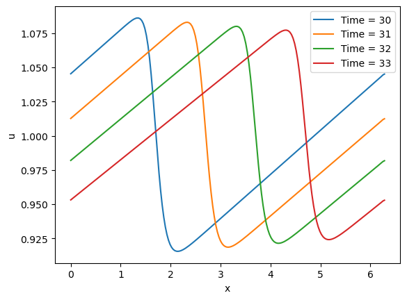
It looks like our fronts travel about 1 spatial unit per time unit, and so we estimate that the relevant speed scale
If we set , then and the CFL condition tells us that , or that
n_mesh = 300
x = np.linspace(0, 2 * np.pi, n_mesh)
u0 = 1 + np.sin(x)
# dtval = 0.001
dtval = 0.025
# dtval = 0.06
# dtval = 0.1
t = np.arange(0, 50, dtval)

eq = BurgersEquation(x, t, u0)

# integrator = RK4(dt=dtval)
# sol = integrator.integrate(eq, (t[0], t[-1]), u0, t_eval=t)
sol =  RK4(dt=dtval).integrate(eq, (t[0], t[-1]), u0)


# plot with colormap for time
colors = plt.cm.rainbow(np.linspace(0, 1, len(sol.y[::500])))
for i, sol0 in enumerate(sol.y[::500]):
    plt.plot(sol0, color=colors[i])
plt.xlabel('x')
plt.ylabel('u')
plt.show()

plt.imshow(sol.y.T)
fixed_aspect_ratio(1/2)
plt.xlabel('t')
plt.ylabel('x')
plt.show()
/var/folders/79/zct6q7kx2yl6b1ryp2rsfbtc0000gr/T/ipykernel_72552/2355403744.py:65: RuntimeWarning: overflow encountered in multiply
  return self.nu * self._laplacian(u) - u * self._derivative(u)
/var/folders/79/zct6q7kx2yl6b1ryp2rsfbtc0000gr/T/ipykernel_72552/2355403744.py:46: RuntimeWarning: invalid value encountered in subtract
  ddu[1:-1] = (u[2:] - 2 * u[1:-1] + u[:-2]) / self.dx**2
/var/folders/79/zct6q7kx2yl6b1ryp2rsfbtc0000gr/T/ipykernel_72552/2355403744.py:46: RuntimeWarning: invalid value encountered in add
  ddu[1:-1] = (u[2:] - 2 * u[1:-1] + u[:-2]) / self.dx**2
/var/folders/79/zct6q7kx2yl6b1ryp2rsfbtc0000gr/T/ipykernel_72552/2355403744.py:24: RuntimeWarning: invalid value encountered in subtract
  du[1:-1] = (u[2:] - u[:-2]) / (2 * self.dx)
/var/folders/79/zct6q7kx2yl6b1ryp2rsfbtc0000gr/T/ipykernel_72552/2355403744.py:28: RuntimeWarning: invalid value encountered in scalar subtract
  du[0] = (u[1] - u[-1]) / self.dx
/var/folders/79/zct6q7kx2yl6b1ryp2rsfbtc0000gr/T/ipykernel_72552/2355403744.py:29: RuntimeWarning: invalid value encountered in scalar subtract
  du[-1] = (u[0] - u[-2]) / self.dx
/var/folders/79/zct6q7kx2yl6b1ryp2rsfbtc0000gr/T/ipykernel_72552/2355403744.py:65: RuntimeWarning: invalid value encountered in subtract
  return self.nu * self._laplacian(u) - u * self._derivative(u)
## Calculate CFL condition
c = 1 # wave speed
## Maximum timestep
print('CFL maximum timestep: ', 3 * eq.dx / c)
CFL maximum timestep: 0.06304199304862461
The sparsity pattern of a PDE
When we discretize a PDE into a set of ODE, these ODE have coupling that depends on the geometry of the spatial domain and the discretization scheme. We can think of this relationship as defining a graph relating the various ODE that we are solving. For our finite-differences discretization of the first derivative, the adjacency matrix relating each of the N lattice sites to each other site looks like this:
The boundary conditions manifest as a condition on the first and last rows and columns of this graph. For example, the pattern above assumes that the field is clamped at zero on the boundaries. In the original PDE, this is the condition , while in the spatially-discretized PDE, this corresponds to assuming that any index that reaches past the edges of the discretized domain will find a zero, . However, if we wanted to capture periodic boundary conditions, then we would need to modify this matrix,
We can come up with similar procedures for reflecting or mixed boundary conditions. Since discretization removes explicit spatial variables from the problem, boundary conditions always appear as connectivity conditions on the resulting graph. Notice that our graph is highly sparse, with nonzero elements. This sparsity can be exploited to avoid having to perform the operations that are typically required when working with matrices.
We can also write the second-order finite difference operator in a similar manner to the first-order finite difference operator: $$
$$
Notice that the second-order operator has elements along its diagonal. This is a consequence of the center value appearing in the finite difference approximation of teh second derivative.
Burgers’ equation in the spectral basis
Recall that our central idea is to convert PDEs into a series of coupled ODES, and then solve this separately. Discretizing space is one way to do this. Each of the resulting ODEs describes a small, contiguous region of the domain.
However, we are free to pick other methods of partitioning the domain. An common alternative is to discretized our field by projecting it onto a series of basis functions defined over the entire domain. If we think of the full spatial solution of a PDE as a superposition of many basis functions, the corresponding coupled ODEs describe the amplitude of each basis function over time.
A common example in classical physics is travelling waves. A sinusoidal travelling wave can be writted as a sum of two standing waves, whose relative amplitudes are each changing over time.
For Burgers’ equation, our original PDE was
Let’s define a set of Fourier basis functions,
where the angular wavenumber parametrizes the basis set. If our domain is , then the values of become a countable set of frequencies that satisfy the periodic boundary conditions, . The Fourier basis functions are orthonormal, so we can write the solution as a linear combination of the basis functions
where is the amplitude of the th Fourier mode at time .
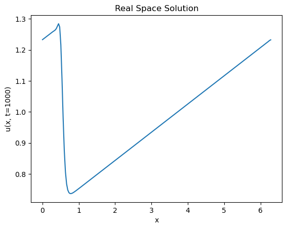
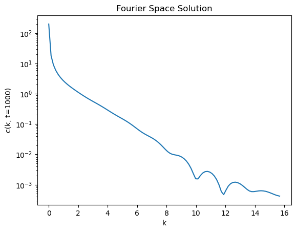
Let’s see what the profile of the Fourier basis functions, , looks like at various times. Notice that when we take the Fourier transform in Python, we truncate and take the first part of the array, since the second half is just the negative frequencies. Recall that these exist due to the phase of the complex exponential in the full definition of the Fourier transform. Since we only care about the magnitude of modes, we can just take the first half of the array returned by the Fourier transform.
time_index = 1000 # The timepoint at which we want to plot the solution profile

plt.figure()
plt.plot(x, sol.y[time_index, :])
plt.xlabel('x')
plt.ylabel(f'u(x, t={time_index})')
plt.title("Real Space Solution")


phi = np.fft.fft(sol.y, axis=1) # Take Fourier transform along indicated axis
k = np.fft.fftfreq(n_mesh, d=eq.dx) # Get the wavenumbers

phi = phi[:, :len(k) // 2]
k = k[:len(k) // 2]

plt.figure()
plt.semilogy(k, np.abs(phi[time_index, :]))
plt.xlabel('k')
plt.ylabel(f'c(k, t={time_index})')
plt.title("Fourier Space Solution")
We can now substituting the Fourier series expression for into the Burgers’ equation PDE. We recall our rules for the Fourier transform of the derivatives of a function, which allow us to write the derivatives of in terms of the amplitudes and wavenumbers of the Fourier modes
Substituting these into the PDE, we get
Notice that the nonlinear term is a bit more involved, since it involves a product of two sums. If we we working with a linear PDE, we wouldn’t have this complication. For example, if diffusion dominates the dynamics (or ), then we would be able to split this equation term-by-term into a set of coupled ODEs in continuous time
For linear equations like the heat equation, the solution method is extremely simple: convert to the spectral domain, determine the time evolution of the coefficients , and then convert back to the physical domain. The modes of the heat equation are decoupled in the spectral domain, so we can solve the ODEs for each mode independently and very efficiently.
Nonlinear terms require pseudospectral methods
For nonlinear systems like Burgers’ equation or reaction-diffusion equations, it’s often not possible to convert the entire PDE into a concise spectral form. Instead, we need to “roundtrip” the solution between the physical and spectral domains at every evaluation. This is a bit more complicated, but it’s still possible to solve the problem efficiently. Methods that involve a roundtrip between the physical and spectral domains are called pseudo-spectral methods.
import numpy as np
from scipy.integrate import solve_ivp

class BurgersEquationSpectral:
    """
    An implementation of the Burgers' equation using spectral methods in Fourier space.

    The user specifies the domain x, time points t, real-spece initial condition u0,
    and the viscosity nu. The class handles converting the initial condition to Fourier
    space, performing the integration in Fourier space, and converting the final
    solution back to real space.
    """

    def __init__(self, x, t, u0, nu=1e-2):
        self.x = x
        self.t = t
        self.u0 = u0
        self.nu = nu
        self.dx = x[1] - x[0]

        # Fourier wavenumbers
        self.k = 2 * np.pi * np.fft.fftfreq(len(x), d=self.dx)
        self.k[0] = 1e-16  # avoid division by zero

        # Fourier transform of initial condition
        self.u0_hat = np.fft.fft(u0)

    def rhs_fourier(self, t, u_hat):
        # Inverse FFT to get u in real space
        u = np.fft.ifft(u_hat)

        # Compute derivatives in Fourier space
        u_x_hat = 1j * self.k * u_hat
        u_xx_hat = -self.k**2 * u_hat

        # Compute nonlinear term (u * u_x) in real space, then transform to Fourier space
        nonlinear_term = u * np.fft.ifft(u_x_hat)
        nonlinear_term_hat = np.fft.fft(nonlinear_term)

        # Compute the right-hand side in Fourier space
        rhs_hat = self.nu * u_xx_hat - nonlinear_term_hat
        return rhs_hat

    def solve(self):
        # Integrate in Fourier space using solve_ivp
        solution = solve_ivp(
            fun=self.rhs_fourier,
            t_span=(self.t[0], self.t[-1]),
            y0=self.u0_hat,
            t_eval=self.t,
            method='RK45'
        )

        # Convert solution back to real space
        u_sol = np.fft.ifft(solution.y, axis=0).real
        return u_sol

# Usage example
x = np.linspace(0, 2 * np.pi, 300)
t = np.linspace(0, 50, 800)
u0 = 1 + np.sin(x)

# Initialize and solve the Burgers' equation
eq = BurgersEquationSpectral(x, t, u0)
sol = eq.solve()


# plot with colormap for time
colors = plt.cm.rainbow(np.linspace(0, 1, len(sol[:, ::100].T)))
for i, sol0 in enumerate(sol[:, ::100].T):
    plt.plot(x, sol0, color=colors[i])
plt.show()


plt.imshow(sol)
fixed_aspect_ratio(1/2)
plt.xlabel('t')
plt.ylabel('x')
plt.show()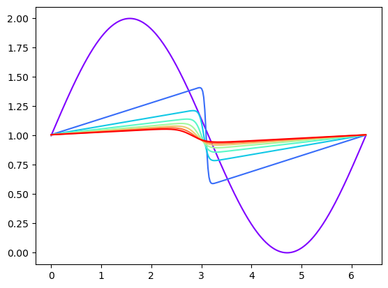
Spectral methods as preconditioning
Recall that the convergence time of linear dynamical systems was related to the condition number of the matrix. That’s because high-condition number matrices are closer to having degenerate column spaces, and thus act like lower-dimensional dynamical systems under repeated iteration. As a result, iterative algorithms like the power method are affected by a matrix’s condition number.
We can think of spectral methods as a way of preconditioning the system, by transforming the system into a basis where the condition number is lower. This is why spectral methods are so effective for linear partial differential equations. For nonlinear PDEs, the condition number of the system is not the only factor that determines the convergence time, but spectral transforms can sometimes allow us to solve the problem with larger timesteps.
What are the appropriate basis functions?
Usually, we pick basis functions that form an orthogonal set, and which are consistent with our boundary conditions. This is because we want to be able to represent the solution as a linear combination of the basis functions, and overlapping basis functions leads to degeneracy. Additionally, orthogonal basis functions usually lead to sparse coupling among the ODEs describing our discretized PDE.
So far, we’ve been using the Fourier basis functions, which describe systems with periodic boundary conditions. However, we can also use other basis functions, which describe systems with different boundary conditions.
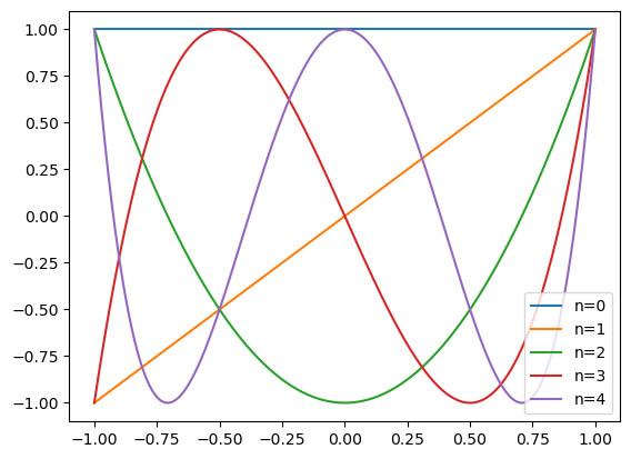
Chebyshev basis functions
For Dirichlet boundary conditions (where the field value is clamped at a constant value at the boundary), we can use the Chebyshev basis functions, which are a set of functions that vanish or approach constant values at the boundary. The Chebyshev basis functions are a set of orthogonal functions that are defined on the interval . They are defined recursively as
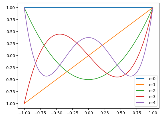
Legendre basis functions
Another option for Dirichlet boundary conditions, are the Legendre basis functions, which are a set of functions that vanish or approach constant values at the boundary. The Legendre basis functions are a set of orthogonal functions that are defined on the interval . They are defined recursively as
### Plot example Chebyshev polynomials

from scipy.special import eval_chebyt

x = np.linspace(-1, 1, 1000)
for n in range(5):
    plt.plot(x, eval_chebyt(n, x), label=f'n={n}')

plt.legend()
plt.show()
### Plot example Legendre polynomials

from scipy.special import eval_legendre

x = np.linspace(-1, 1, 1000)
for n in range(5):
    plt.plot(x, eval_legendre(n, x), label=f'n={n}')

plt.legend()
plt.show()
Some specificities of Burgers’ equation
In Burgers’ equation, the shock waves are discontinuities in the derivative of the velocity, but not in the density. As with other PDEs with predominant advection, the shock waves propagate ballistically, i.e. at a constant speed of sound in the fluid. As a result, when the diffusion term is weak () certain initial conditions in the shape of a shock wave will get carried with the flow, and will not change shape,
Burgers’ equation is a unique nonlinear PDE because it can be transformed into a linear PDE by introducing a new set of coordinates. The Cole-Hopf transformation consists of substituting the variable with using the following defintion
Inserting this into the viscous Burgers equation gives
After some algebraic manipulation, we get
This is a linear diffusion equation, which can easily be solved in one dimension. We can solve this simplified heat equation, and then cast back into the original variables by performing the inverse transformation
Unlike our chaotic systems, the complexity of the dynamics of the Burgers equation is not intrinsic, but rather due to our choice of dynamical variables. This is a preview of a common problem we will encounter in machine learning: is a problem intrinsically hard, or do we just need to pick the right coordinates?
Appendix
This is William’s leftover code, which might get used in a future version of the tutorial
# Solve the KuramotoSivashinsky equation with spectral methods

from scipy.integrate import solve_ivp

class KuramotoSivashinskyEquationSpectral:

    def __init__(self, x, t, u0, nu=1.0):
        self.x = x
        self.t = t
        self.u0 = u0
        self.nu = nu

    def rhs(self, t, u):
        u = u.reshape((len(self.x), 1))
        du = np.fft.fft(u, axis=0)
        ddu = np.fft.fft(du, axis=0)
        return -self.nu * du + ddu

    def solve(self):
        u0 = np.fft.fft(self.u0)
        sol = solve_ivp(self.rhs, (self.t[0], self.t[-1]), u0, t_eval=self.t)
        return np.real(np.fft.ifft(sol.y, axis=0))
import numpy as np
from scipy.integrate import solve_ivp

class KuramotoSivashinskySpectral:
    """
    u_t = - u u_x - nu*u_xx - u_xxxx  (periodic on [0, L))
    """
    def __init__(self, x, t, u0, nu=1.0):
        self.x = x
        self.t = t
        self.u0 = np.asarray(u0, dtype=float)
        self.nu = float(nu)

        self.N = len(x)
        self.L = x[-1] - x[0] + (x[1] - x[0])  # domain length assuming uniform grid
        self.dx = self.L / self.N

        # Angular wavenumbers (derivative: d/dx -> i*k)
        self.k = 2.0 * np.pi * np.fft.fftfreq(self.N, d=self.dx)
        self.ik = 1j * self.k
        self.k2 = self.k**2
        self.k4 = self.k**4

        # Linear operator in Fourier space from: -nu*u_xx - u_xxxx
        #  -> (+nu*k^2 - k^4) * u_hat
        self.Lop = self.nu * self.k2 - self.k4

        # 2/3 de-aliasing mask (keep lowest 2/3 modes)
        cut = self.N // 3
        mask = np.zeros(self.N, dtype=bool)
        if cut > 0:
            mask[:cut] = True
            mask[-cut:] = True
        # always keep k=0
        mask[0] = True
        self.dealias = mask

    def rhs(self, t, u_hat):
        # u_hat is Fourier state; compute nonlinear term in physical space
        u = np.fft.ifft(u_hat)                  # real-space field
        u2_hat = np.fft.fft(u * u)              # FFT(u^2)
        u2_hat *= self.dealias                  # 2/3 de-aliasing

        # Nonlinear term: - (1/2) * i*k * FFT(u^2)
        N_hat = -0.5 * self.ik * u2_hat

        # Total RHS in Fourier space
        return self.Lop * u_hat + N_hat

    def solve(self, method="RK45", rtol=1e-6, atol=1e-9):
        # Initialize in Fourier space
        u0_hat = np.fft.fft(self.u0.astype(complex))

        sol = solve_ivp(
            fun=self.rhs,
            t_span=(self.t[0], self.t[-1]),
            y0=u0_hat,
            t_eval=self.t,
            method=method,
            rtol=rtol,
            atol=atol,
            vectorized=False,
        )

        # Back to real space: shape (N, T)
        U = np.fft.ifft(sol.y, axis=0).real
        return U

# ---- Example usage ----
# Use endpoint=False for a clean periodic grid (no duplicate point)
x = np.linspace(0, 2*np.pi, 300, endpoint=False)
t = np.linspace(0, 50, 200)
u0 = 1 + np.sin(x)

eq = KuramotoSivashinskySpectral(x, t, u0, nu=1.0)
U = eq.solve(method="RK45")  # "BDF" can be more stable for stiff cases

plt.figure()
plt.plot(x, U[:, 0], label='t = %.2f' % t[0])
plt.plot(x, U[:, -1], label='t = %.2f' % t[-1])
plt.xlabel('x')
plt.ylabel('u(x,t)')
plt.legend()
plt.tight_layout()
plt.show()
---------------------------------------------------------------------------
KeyboardInterrupt                         Traceback (most recent call last)
Cell In[63], line 77
     74 u0 = 1 + np.sin(x)
     76 eq = KuramotoSivashinskySpectral(x, t, u0, nu=1.0)
---> 77 U = eq.solve(method="RK45")  # "BDF" can be more stable for stiff cases
     79 plt.figure()
     80 plt.plot(x, U[:, 0], label='t = %.2f' % t[0])

Cell In[63], line 55, in KuramotoSivashinskySpectral.solve(self, method, rtol, atol)
     51 def solve(self, method="RK45", rtol=1e-6, atol=1e-9):
     52     # Initialize in Fourier space
     53     u0_hat = np.fft.fft(self.u0.astype(complex))
---> 55     sol = solve_ivp(
     56         fun=self.rhs,
     57         t_span=(self.t[0], self.t[-1]),
     58         y0=u0_hat,
     59         t_eval=self.t,
     60         method=method,
     61         rtol=rtol,
     62         atol=atol,
     63         vectorized=False,
     64     )
     66     # Back to real space: shape (N, T)
     67     U = np.fft.ifft(sol.y, axis=0).real

File ~/mamba/envs/cphy/lib/python3.13/site-packages/scipy/integrate/_ivp/ivp.py:655, in solve_ivp(fun, t_span, y0, method, t_eval, dense_output, events, vectorized, args, **options)
    653 status = None
    654 while status is None:
--> 655     message = solver.step()
    657     if solver.status == 'finished':
    658         status = 0

File ~/mamba/envs/cphy/lib/python3.13/site-packages/scipy/integrate/_ivp/base.py:197, in OdeSolver.step(self)
    195 else:
    196     t = self.t
--> 197     success, message = self._step_impl()
    199     if not success:
    200         self.status = 'failed'

File ~/mamba/envs/cphy/lib/python3.13/site-packages/scipy/integrate/_ivp/rk.py:144, in RungeKutta._step_impl(self)
    141 h = t_new - t
    142 h_abs = np.abs(h)
--> 144 y_new, f_new = rk_step(self.fun, t, y, self.f, h, self.A,
    145                        self.B, self.C, self.K)
    146 scale = atol + np.maximum(np.abs(y), np.abs(y_new)) * rtol
    147 error_norm = self._estimate_error_norm(self.K, h, scale)

File ~/mamba/envs/cphy/lib/python3.13/site-packages/scipy/integrate/_ivp/rk.py:64, in rk_step(fun, t, y, f, h, A, B, C, K)
     62 for s, (a, c) in enumerate(zip(A[1:], C[1:]), start=1):
     63     dy = np.dot(K[:s].T, a[:s]) * h
---> 64     K[s] = fun(t + c * h, y + dy)
     66 y_new = y + h * np.dot(K[:-1].T, B)
     67 f_new = fun(t + h, y_new)

File ~/mamba/envs/cphy/lib/python3.13/site-packages/scipy/integrate/_ivp/base.py:154, in OdeSolver.__init__.<locals>.fun(t, y)
    152 def fun(t, y):
    153     self.nfev += 1
--> 154     return self.fun_single(t, y)

File ~/mamba/envs/cphy/lib/python3.13/site-packages/scipy/integrate/_ivp/base.py:23, in check_arguments.<locals>.fun_wrapped(t, y)
     22 def fun_wrapped(t, y):
---> 23     return np.asarray(fun(t, y), dtype=dtype)

Cell In[63], line 41, in KuramotoSivashinskySpectral.rhs(self, t, u_hat)
     39 def rhs(self, t, u_hat):
     40     # u_hat is Fourier state; compute nonlinear term in physical space
---> 41     u = np.fft.ifft(u_hat)                  # real-space field
     42     u2_hat = np.fft.fft(u * u)              # FFT(u^2)
     43     u2_hat *= self.dealias                  # 2/3 de-aliasing

File ~/mamba/envs/cphy/lib/python3.13/site-packages/numpy/fft/_pocketfft.py:314, in ifft(a, n, axis, norm, out)
    312 if n is None:
    313     n = a.shape[axis]
--> 314 output = _raw_fft(a, n, axis, False, False, norm, out=out)
    315 return output

File ~/mamba/envs/cphy/lib/python3.13/site-packages/numpy/fft/_pocketfft.py:94, in _raw_fft(a, n, axis, is_real, is_forward, norm, out)
     90 elif ((shape := getattr(out, "shape", None)) is not None
     91       and (len(shape) != a.ndim or shape[axis] != n_out)):
     92     raise ValueError("output array has wrong shape.")
---> 94 return ufunc(a, fct, axes=[(axis,), (), (axis,)], out=out)

KeyboardInterrupt: