Martingales and the Brownian Bridge - Computational Physics

Instructions on using Jupyter Notebooks¶

Using a Jupyter Notebook. After opening a Jupyper notebook in an editing environment (local or a cloud-hosted environment), no variables or functions are present in the namespace. As cells in the notebook are run, variables and functions become part of the namespace and are now usable in later cells. If you restart the notebook, the namespace is cleared and you will need to re-run cells to reinitialize any functions or variables needed for later cells

Running the cells below will run a “preamble,” which imports external packages and code into the Jupyter Notebook environment. This includes external Python libraries, as well as internal code on which

Preamble¶

Before writing any code, we will load several packages into the notebook environment.

matplotlib - a plotting library
numpy - a library implementing numerical operations on arrays
scipy - a general scientific computing library

A note on cloud-hosted notebooks. If you are running a notebook on a cloud provider, such as Google Colab or CodeOcean, remember to save your work frequently. Cloud notebooks will occasionally restart after a fixed duration, crash, or prolonged inactivity, requiring you to re-run code.

Open this notebook in Google Colab:

import numpy as np
import matplotlib.pyplot as plt
%matplotlib inline

The Brownian Bridge¶

A Brownian bridge is a stochastic process describing Brownian motion that is “pinned” to start and end at fixed values over a fixed interval. Unlike standard Brownian motion, which can wander anywhere in finite time, the Brownian bridge describes the subset of all possible random walks that start and end at the clamped values on either end.

One system that can be approximated by a Brownian bridge is the random motion of biological polymers, like DNA, which are confined to a fixed length. In such systems, the polymer’s configuration fluctuates randomly in the interior, but the two ends are constrained---either by being chemically bound, as in circular DNA, or by attachment to fixed sites within a cell.

We will use the notation $\{W(t): 0 \leq t \leq 1\}$ to describe standard Brownian motion on an interval of length 1, and the Brownian bridge $\\{B(t): 0 \leq t \leq 1\\}$ is defined as a Brownian bridge that starts and ends at zero.

Simulating a Brownian bridge¶

Naively, we can approximate a Brownian bridge by simulating a huge number of standard Brownian motion trajectories starting at zero when $t=0$ , and then selecting the subset of trajectories that reach 0 at $t=1$ . This represents a form of rejection sampling.

The martingale property¶

Classical Brownian motion is a martingale. This means that the expected value of the process at any future time is equal to the current value. We can write this as

\mathbb{E}[W(t + \tau)] = W(t), \qquad \tau > 0.

(1)

For classical Brownian motion, the variance of the process at any future time is therefore equal to the current time. We can write this as

\mathrm{Var}(W(t)) = t.

(2)

Intuitively, the martingale property implies that variance must increase over time, beause the variance of each step is constant. However, the variance of a Brownian bridge does not continuously increase over time. For example, at $t=0$ and $t=1$ , the variance is zero because all walks have the same starting and ending values. The Brownian bridge is thus a non-martingale.

If we wanted to transform standard Brownian motion into a Brownian bridge, we could do so by subtracting the term $t W(1)$ from the process. This would give us a process that starts and ends at zero, but is not a martingale.

\mathbb{E}[B(t)] = B(t) - t W(1).

(3)

$B(t)$ is an example of a Gaussian process. A Gaussian process is a collection of random variables, any finite number of which have a joint Gaussian distribution. The distribution of the Brownian bridge at a fixed time $t$ is Gaussian with mean 0 and variance $t(1-t)$ .

B(t) \sim \mathcal{N}\big(0, \, \sqrt{t(1-t)}\big).

(4)

To Do¶

Please complete the following exercises. For the free response questions, please write your answer in the cell below the question. Depending on the version of the course, the instructor solutions may be available for you to use to test your code in case you get stuck. However, you need to fill in and run your own code and free response answers. For the free response, you can edit a cell by double-clicking on it in your notebook editor. Running this text cell will re-render the text and LaTeX to include your answers.

Implement the rejection sampling method for the Brownian bridge. You will need to use np.random.normal to sample steps from the normal distribution. In the rejection sampling method, we simulate a large number n_rejections of standard Brownian motion trajectories that start at 0, and we then select the single trajectory that ends closest to 0 at time $t=1$ . Below, you will see starter code for implementing BridgeBaseClass and BrownianBridgeRejection. Fill in the missing methods, and then run the included code snippet belowto generate and plot multiple random instances of the Brownian bridge.

    Your Answer: complete the code below

Implement an improved Brownian bridge simulator using the transformation of standard Brownian motion described above. Below, you will see starter code for BrownianBridgeTransform. Fill in the missing methods, and then run the included code snippet below to generate and plot multiple random instances of the Brownian bridge.

    Your Answer: complete the code below

Using the code snippet provided below, check that the the properties of the your new Brownian bridge implementation (Gaussian distribution, zero mean, changing variance) are all satisfied. How can you improve the agreement between the theoretical and empirical results?

    Your Answer:

If you look at the API reference for numpy.random.normal, you can see that there are many other distributions that we can instead sample our random steps from. Try a different distribution, and see how it affects the results. Does it match your intuition? Does it still satisfy the martingale property?

    Your Answer:

The casino game blackjack is a martingale when played under perfectly-fair conditions. However, in practice, the house edge is always positive, and the game is no longer a martingale. Why is this?

    Your Answer:


class BridgeBaseClass:
    """
    Simulate a stochastic process that is pinned to start and end at fixed values 
    over a fixed interval.

    Parameters
        T (float): The total time of the simulation.
        a (float): The starting value of the process.
        b (float): The ending value of the process.
    """

    def __init__(self, T=1.0, a=0.0, b=0.0):
        self.T = T
        self.a = a
        self.b = b

    def simulate(self, n_steps):
        """Implement the simulation method. This is a placeholder for the actual 
        implementation, which will be overridden for each subclass."""
        pass


class BrownianBridgeRejection(BridgeBaseClass):
    """
    Simulate a Brownian bridge by rejection sampling.

    Parameters
        n_rejections (int): The number of rejection samples to take.
        *args, **kwargs: Additional arguments to pass to the parent class.
    """

    def __init__(self, n_rejections, *args, **kwargs):
        super().__init__(*args, **kwargs)
        self.n_rejections = n_rejections

    def simulate(self, n_steps):
        """Simulate a Brownian bridge.
        
        Args:
            n_steps (int): The number of steps to simulate.

        Returns
            np.ndarray: A 1D array of shape (n_steps) containing the simulated 
                Brownian bridge.
        """
        ########## YOUR CODE HERE ##########
        #
        # YOUR CODE HERE
        #
        ########## YOUR CODE HERE ##########
        raise NotImplementedError()
    

class BrownianBridgeTransform(BridgeBaseClass):
    """
    Simulate a Brownian bridge by using a transformation of standard Brownian motion.
    """

    def __init__(self, *args, **kwargs):
        super().__init__(*args, **kwargs)

    def simulate(self, n_steps):
        """Simulate a Brownian bridge using a transformation of standard Brownian motion."""
        ########## YOUR CODE HERE ##########
        #
        # YOUR CODE HERE
        #
        ########## YOUR CODE HERE ##########
        raise NotImplementedError()

Test and use your code¶

You don’t need to write any code below, these cells are just to confirm that everything is working and to play with your implementation
If you are working from a local fork of the entire course, then you may already have access to the instructorsolutions. In this case, make sure to git pull to make sure that you are up-to-date (save your work first).
If you are working from a single downloaded notebook, or are working in Google Colab, then you will need to manually download the solutions files from the course repository. The lines below will do this for you, but if they fail you will need to manually download the file from the course repository and place it in the solutions directory.
Depending on your version of the course and textbook, the instructor solutions may be available to for you to use, particularly for testing in case you get stuck. However, you need to fill in and run your own code and free response answers. If you are running the code from the instructor solutions, you will see a message printed to the output of the cells below.

## If available, download instructor solutions
import os
import requests
# Check if the "solutions" directory exists. If not, create it and download the solution file
if not os.path.exists('solutions'):
    os.makedirs('solutions')
else:
    print('Directory "solutions" already exists. Skipping creation.')

# Now download the solution file into the directory we just created
url = 'https://raw.githubusercontent.com/williamgilpin/cphy/main/hw/solutions/brownian_bridge.py'
response = requests.get(url)
file_path = os.path.join('solutions', 'brownian_bridge.py')
if not os.path.exists(file_path):
    with open(file_path, 'wb') as file:
        file.write(response.content)
    print(f'File saved to {file_path}')
else:
    print(f'File already exists at {file_path}, not overwritten.')

## import Instructor's solutions
# from solutions.brownian_bridge import BrownianBridgeTransform, BrownianBridgeRejection

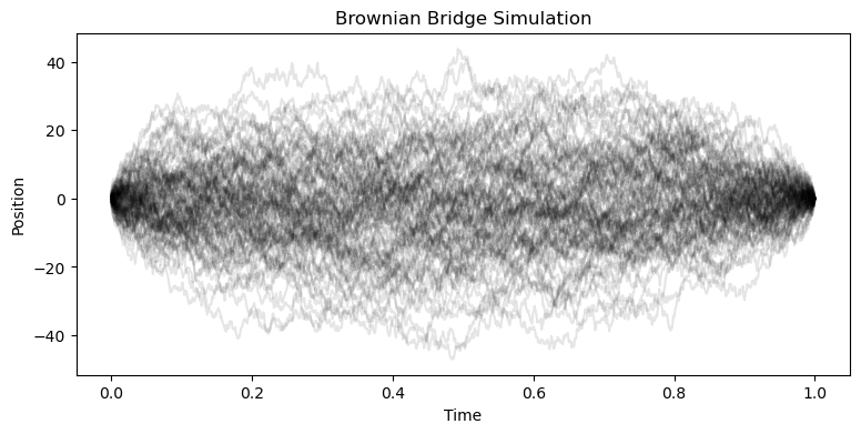
bridge = BrownianBridgeRejection(n_rejections=1000, T=1.0, a=0.0, b=0.0)

## Simulate many bridges and plot them
all_bridges = [bridge.simulate(1000) for _ in range(100)]
time_vals = np.linspace(0, bridge.T, 1000)

plt.figure(figsize=(9, 4))
plt.plot(time_vals, np.array(all_bridges).T, color='black', alpha=0.1);
plt.xlabel('Time')
plt.ylabel('Position')
plt.title('Brownian Bridge Simulation')
plt.show()

Running with Instructor Solutions. If you meant to run your own code, do not import from solutions

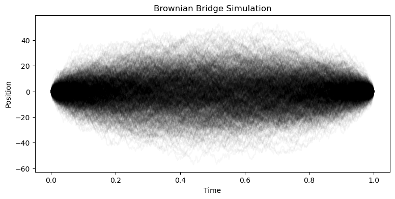
bridge = BrownianBridgeTransform(T=1.0, a=0.0, b=0.0)

## Simulate many bridges and plot them
all_bridges = [bridge.simulate(1000) for _ in range(1000)]
all_bridges = np.array(all_bridges)
time_vals = np.linspace(0, bridge.T, 1000 + 1)

plt.figure(figsize=(9, 4))
plt.plot(time_vals, all_bridges.T, color='black', alpha=0.03);
plt.xlabel('Time')
plt.ylabel('Position')
plt.title('Brownian Bridge Simulation')
plt.show()

fig, axes = plt.subplots(5, 1, figsize=(6, 12), sharex=True)
time_indices = [0, 10, 50, 90, 100]
for ax, idx in zip(axes, time_indices):
    ax.hist(all_bridges[:, idx], alpha=0.5)
    # ax.set_ylabel(f"t={time_vals[idx]:.2f}")
    ax.annotate(f"t={time_vals[idx]:.2f}", xy=(0.95, 0.85),
                 xycoords="axes fraction", ha="right", va="top")
axes[-1].set_xlabel("Value")
plt.tight_layout()
plt.show()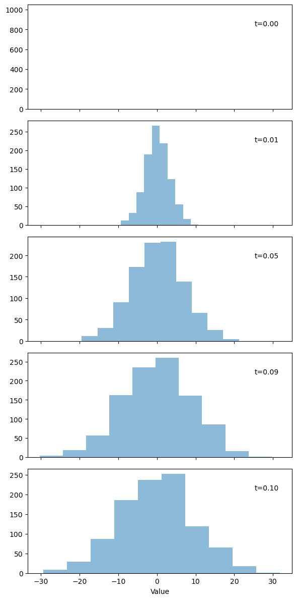

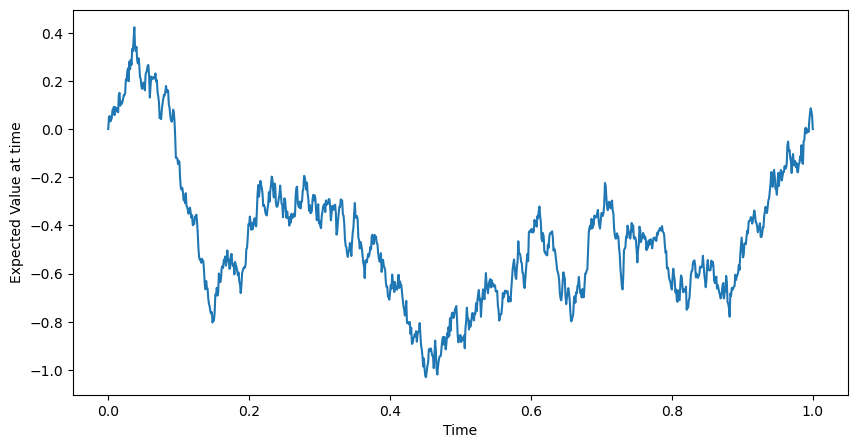
## check expected mean
plt.figure(figsize=(10, 5))
plt.plot(time_vals, np.mean(all_bridges, axis=0))
plt.xlabel('Time')
plt.ylabel('Expected Value at time')

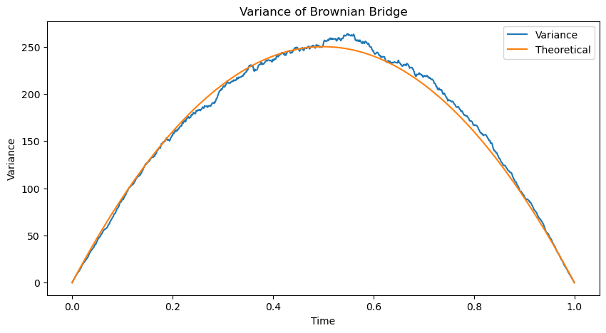
## check variance
plt.figure(figsize=(10, 5))
plt.plot(time_vals, np.var(all_bridges, axis=0))
plt.plot(time_vals, time_vals * (1 - time_vals) * 1000)
plt.legend(['Variance', 'Theoretical'])
plt.xlabel('Time')
plt.ylabel('Variance')
plt.title('Variance of Brownian Bridge')
plt.show()

Chapters

Unsupervised learning: Clustering

Homework

Graph traversal, cellular automata, and percolation