Runtime complexity, Recursion, and estimating Feigenbaum's constant for chaos
Preamble: Run the cells below to import the necessary Python packages
This notebook created by William Gilpin. Consult the course website for all content and GitHub repository for raw files and runnable online code.
import numpy as np

from IPython.display import Image, clear_output, display

# Import local plotting functions and in-notebook display functions
import matplotlib.pyplot as plt
%matplotlib inline
Finding bifurcations in the logistic map
In previous lectures we saw how to use the logistic map to model population growth. We also saw that the logistic map can exhibit chaotic behavior for certain values of the parameter $r$.
In this lecture we will explore the behavior of the logistic map in more detail. In particular, we will examine more closely how the behavior of the logistic map changes as we vary the parameter $r$.
Re-implementing the logistic map with classes
First we will implement two classes: One that represents the logistic map, and one that calculates its bifurcation diagram. Unlike previous lectures, we will implement the Logistic map using an iterable class.
Special methods in Python classes: Python reserves certain method names for special purposes. For example, the __init__ method is automatically called when an object is created. The __str__ method is called when an object is printed. The __call__ method allows an object to be treated like a function.
class LogisticMap:
    """
    Implements the logistic map.

    Attributes:
        r (float): The growth rate parameter
        x (float): The current value of x for the logistic map.
    """

    def __init__(self, r=3.8, x0=0.65):
        self.r = r
        self.x = x0

    def next(self):
        """Compute the next value of the map."""
        self.x = self.r * self.x * (1 - self.x)
        return self.x

    def simulate(self, n):
        """Simulate the map for n iterations."""
        x = []
        for _ in range(n):
            x.append(self()) # Notice that we can call the class like a function
        return x

    # The __call__ method allows us to call an instance of this class like a function.
    # It must return the value that should be returned when the instance is called.
    def __call__(self):
        self.x = self.r * self.x * (1 - self.x)
        return self.x
        # print("don't dp this")
        return self.next()

    # The __str__ method is called when the object is printed. It must return a string.
    def __str__(self):
        return 'Logistic map with r = {:.2f}'.format(self.r)


map = LogisticMap()

# invoke the special __string__ method
print(map)

# # one step of the map
print(f"Initial condition: {map.x}")
print(f"First iteration: {map()}")

# # plot the trajectory
traj = map.simulate(1000)
plt.figure(figsize=(9, 6))
plt.plot(traj)
plt.xlim(0, len(traj))
plt.xlabel('Iteration')
plt.ylabel('x')
Logistic map with r = 3.80
Initial condition: 0.65
First iteration: 0.8644999999999998
Text(0, 0.5, 'x')

Iterable objects in Python: Python has a special protocol for objects that can be used in for loops, or implicitly in list comprehensions. An object is iterable if it has a special method called __iter__ that returns an object with a method called __next__.
We will use these methods to implement a class that finds the bifurcation diagram of the logistic map.
class BifurcationDiagram:
    """
    Find the bifurcation diagram for a map using __iter__ in Python. This stateful
    implementation is more efficient than the stateless implementation we used previously,
    because it does not need to store the entire trajectory in memory.

    We will iterate over the map, one value of r at a time, and plot the last
    values of x for each value of r after a transient has elapsed

    Attributes:
        dmap (callable): A discrete map object. Must contain a simulate method that returns a
            trajectory of the map.
        rmin (float): The minimum value of r to use.
        rmax (float): The maximum value of r to use.
        rsteps (int): The number of steps to take between rmin and rmax.
        n (int): The number of iterations to use for each value of r.
        transient (int): The number of iterations to discard as transient.

    """

    def __init__(self, dmap, rmin, rmax, rsteps, n, transient=100):
        self.dmap = dmap
        self.rmin = rmin
        self.rmax = rmax
        self.rsteps = rsteps
        self.n = n
        self.transient = transient

    # The __iter__ method makes this class iterable. It must return an object
    # that implements the __next__ method. Iterable objects can be used in for
    # loops and list comprehensions.
    def __iter__(self):
        return self

    # The __next__ method is called by the for loop to get the next item in the
    # iteration. It must return the next item, or raise StopIteration if there
    # are no more items.
    def __next__(self):

        # Set map to use the current value of r
        self.dmap.r = self.rmin

        # Stop the calculation if we have reached the end of the parameter interval
        if self.rmin > self.rmax:
            raise StopIteration

        ## Otherwise, simulate the map for nsteps at the current value of r, and return
        ## the last values after the transient
        else:
            r = self.rmin
            self.rmin += self.rsteps
            return self.dmap.simulate(self.n)[self.transient:], r
## Instantiate a bifurcation diagram for the logistic map
diagram = BifurcationDiagram(LogisticMap(),  2.4, 4.0, 0.001, 1000)

plt.figure(figsize=(9, 6))

## We can iterate over the diagram object itself to get the values of r and x
# for i in range(10):
#     print(i)
for traj, r in diagram:
    plt.plot([r] * len(traj), traj, ',k', alpha=0.25)

plt.xlabel('r')
plt.ylabel('x')
plt.xlim(2.4, 4.0)
(2.4, 4.0)

How often does the logistic map undergo period doubling?
When does the logistic map undergo period doubling? On the bifurcation diagram, we see that the period doubles at certain values of $r$. Initially, these values are spaced pretty far apart in $r$, but as we move to the right on the bifurcation diagram, the values of $r$ at which the period doubles get closer and closer together.
We want to find these exact values of $r$ at which the period doubles. We will use a variety of search algorithms to find these values.
Our code will consist of two parts:
- A "check" function that determines whether the period of the logistic map has doubled. This will take two trajectories corresponding to two different values of $r$ and determine whether the period has doubled by comparing the two trajectories.
- A "search" function that uses the "check" function to find the values of $r$ at which the period doubles.
# naive search: line scan

def check_period_doubling(prev_traj, current_traj, tolerance=0.3):
    """
    Check if the period has doubled from the previous trajectory to the current
    trajectory. Uses a basic test of whether the number of unique values in the
    current trajectory is greater than the number of unique values in the previous
    trajectory.

    Args:
        prev_traj (array): Previous trajectory
        current_traj (array): Current trajectory
        tolerance (float): How close the period doubling ratio must be to 2 in order to
            be considered a period doubling event.

    Returns:
        bool: True if period doubled, False otherwise
    """

    # Round each trajectory to 4 decimal places to avoid numerical errors, and then
    # count the number of unique values seen. A period 2 orbit will have 2 unique
    # values, a period 4 orbit will have 4 unique values, and so on.
    prev_unique_vals = len(set(np.round(prev_traj, decimals=4)))
    current_unique_vals = len(set(np.round(current_traj, decimals=4)))

    # Check to see if the number of unique values has doubled, to within a threshold
    has_doubled = np.abs(current_unique_vals / prev_unique_vals - 2) < tolerance
    # has_doubled = (current_unique_vals == 2 * prev_unique_vals)
    return has_doubled


def line_scan(dmap, rmin, rmax, n_rvals=100, transient=50):
    """
    Find the doubling points for a map using a line scan

    Scan the values of r between rmin and rmax and find the values of r where the
    map doubles in period. This function uses the discrete map's simulate method
    to generate a trajectory for each value of r.

    Args:
        dmap (object): A discrete map object. Must contain a simulate method that
            returns a trajectory of the map.
        rmin (float): The minimum value of r to use.
        rmax (float): The maximum value of r to use.
        n_rvals (int): The number of values of r to use between rmin and rmax.
        transient (int): The number of iterations to discard as transient.

    Returns:
        array: An array of values of r where the map doubles in period.

    """
    ## Create an array of r values to scan over
    rvals = np.linspace(rmin, rmax, n_rvals)
    doubling_rvals = []
    prev_traj = None
    for r in rvals:

        ## Set the parameter value and simulate the map in order to get a trajectory
        dmap.r = r
        traj = np.array(dmap.simulate(1000)[-transient:])

        # If we have a previous trajectory, check for period doubling. If it
        # has doubled, add the current value of r to the list of doubling r values
        if prev_traj is not None:
            if check_period_doubling(prev_traj, traj):
                doubling_rvals.append(r)

        ## Update the previous trajectory
        prev_traj = traj

    return np.array(doubling_rvals)


import time

start = time.time()
rvals_c = line_scan(LogisticMap(), 2.4, 3.57, n_rvals=300)
print(rvals_c)
end = time.time()
print(f"Time elapsed: {end - start} seconds")

# # filter out values that change by less than 0.01
# rvals_c = rvals_c[:-1][np.diff(rvals_c) > (3.6 - 2.4) / (1000 - 1)]


# plt.figure()
# gaps = rvals_c[1:] - rvals_c[:-1]
# plt.plot(gaps)
# print(gaps[:-1] / gaps[1:])

# vals = [3.0]
# gap = 0.45252525
# for i in range(5):
#     nxt = vals[-1] + gap
#     vals.append(nxt)
#     gap = gap / 4.667
# rvals_c = np.array(vals)
# gaps = rvals_c[1:] - rvals_c[:-1]
# plt.plot(gaps)
[2.99869565 3.44869565 3.54652174 3.56608696]
Time elapsed: 0.062246084213256836 seconds
Next, we will plot these values of $r$ in red on the bifurcation diagram, to see whether they look right.
plt.figure(figsize=(9, 6))

## Create and plot the bifurcation diagram
diagram = BifurcationDiagram(LogisticMap(),  2.4, 4.0, 0.001, 1000)
for traj, r in diagram:
    plt.plot([r] * len(traj), traj, ',k', alpha=0.25)

## Draw vertical lines at the period doubling points we found
for r in rvals_c:
    plt.axvline(r, color='r', alpha=0.5)

plt.xlabel('r')
plt.ylabel('x')
# plt.xlim(2.4, 3.6)
plt.xlim(2.8, 3.6)
(2.8, 3.6)

How are these doubling events distributed? We will plot the gaps (in $r$) between successive doubling events to see if they follow a pattern.
# filter out values that change by less than 0.01
# rvals_c = rvals_c[:-1][np.diff(rvals_c) > (3.6 - 2.4) / (10000 - 1)]

plt.figure()
gaps = rvals_c[1:] - rvals_c[:-1]
plt.xlabel('Doubling event index')
# in latex r_c
plt.ylabel('$r^*_{i+1} - r^*_i$')


plt.plot(gaps)
print(f"Ratios between successive doublings: {gaps[:-1] / gaps[1:]}")
Ratios between successive doublings: [4.6 5. ]

This looks reasonable, but we can see from the bifurcation diagram that this isn't super accurate. Can we localize the period doubling events more accurately?
Searching parameter space with binary search
A binary search is a search algorithm that works on a sorted list.
Binary search has runtime cost $\mathcal{O}\left(\log{(N)}\right)$ because it cuts the list in half each time.

def binary_search(a, target):
    """
    Find the index of the first element in a *sorted* array that is greater than or
    equal to the target.

    We are using a two-pointer approach where one pointer is always greater than the
    target and the other is always less than the target. The pointers start at the ends
    of the array and move towards each other until they meet. The index of the left
    pointer is the index of the first element greater than or equal to the target.

    Args:
        a (array): A sorted array of numbers.
        target (float): The target value to search for.

    Returns:
        int: The index of the first element greater than or equal to target.
    """
    lo = 0
    hi = len(a)
    while lo < hi:
        mid = (lo + hi) // 2
        if a[mid] < target:
            lo = mid + 1
        else:
            hi = mid
    return lo

a = np.array([1, 2, 3, 4, 7, 8, 9, 10, 15, 43, 99])

print(binary_search(a, 5))
4
Determining Big-O for an algorithm
- The Big-O notation is a way to describe the runtime and memory complexity of an algorithm. It describes how the runtime of an algorithm scales with the size $N$ of the input.
- $\mathcal{O}(N)$
- $N$ may refer to the number of lattice points when simulating a PDE, the number of timepoints when simulating a dynamical system, the number of bodies in a gravitational simulation, etc. It depends on the problem and the context, but usually it's the "largest" number in the problem.
- In practice, the scaling almost always some combination of a polynomial $N^{\alpha}$ and $\log(N)$. Remember that overwriting values, peeking the front of a queue, etc take constant time or $\mathcal{O}(1)$
Some useful times to know
- $\log{(N)}$ usually means you can quickly rule out large groups of the input (recursion, bisection search, etc)
- $\text{exp}\left(N\right)$ implies a combinatoric explosion as the number of inputs increases, such as a process that branches. This is usually not optimal, but some problems are inherently exponential. An example is the traveling salesman problem, or finding the ground state of a set of $N$ randomly-coupled Ising spins.
- Stirling's approximation: $N! \sim \sqrt{N} e^{-N} N^N$ or $\log{(N!)} \sim N \log{(N)}$
- Sorting a list via mergesort is $\mathcal{O}(N \log(N))$
- Binary search, two-sum are pointers with $\log{(N)}$ time
- Dot product of two length-$N$ vectors is $\mathcal{O}(N)$. $N \times N$ matrix-vector product is $\mathcal{O}(N^2)$. Product of two $N \times N$ matrices is $\mathcal{O}(N^3)$
import timeit
nvals = np.arange(2, 800)

nvals = np.arange(2, 5000, 3)
all_times = list()
for n in nvals:
    all_reps = list()
    all_times.append(
        timeit.timeit(
            "binary_search(np.arange(n), n // 2)", globals=globals(), number=10000
        )
    )

plt.figure(figsize=(9, 6))
plt.plot(nvals, all_times, 'k')
plt.xlabel('n')
plt.ylabel('Time (s)')
Text(0, 0.5, 'Time (s)')

We can see that the runtime of binary search is $\mathcal{O}\left(\log{(N)}\right)$
This is because the algorithm cuts the size of the list in half each time. Since the list is already sorted, we are able to quickly rule out half of the input each time we make a comparison.
We can compare this to our earlier linear linescan search, which has runtime $\mathcal{O}\left(N\right)$.
Improving our calculation of doubling values
Now let's return to our logistic map example. We will use a binary search to find the values of $r$ at which the period doubles. Because binary search avoids scanning many parameter values, we can avoid many intermediate values of $r$ between the doubling events.
Implementing binary search for period doubling
There a are a few nuances to our approach, compared to traditional binary search.
We need to perform a three-pointer comparison among the periods of the logistic map at $r_{min}$, $r_{middle}$, and $r_{max}$. This is because the period doubling may not occur exactly at $r$. We thus implement a three-way comparison function, which requires three trajectories to be passed in, and identifies if the period doubles between the first and second trajectories, or the second and third trajectories.
We need to find several values of $r$ corresponding to critical doubling values, rather than just one value. This requires multiple binary searches over different intervals, as well as a heuristic for modifying the intervals to ensure that we don't repeatedly find the same root. We break down this process as follows:
We search the full $r$ interval.
Upon finding a doubling value, we shrink the interval so that its rightmost value is just below the root we just found by some tolerance $\epsilon$.
We then search the new interval for the next doubling value.
We repeat this process until we have found all the doubling values. This heuristic will fail if the period doubling values are closer than $\epsilon$ apart. In this case, we would need to reduce $\epsilon$ and try again. This same difficulty manifests in methods used to find multiple roots (zero crossings) of continuous functions.
## Three-way comparison function
def check_period_doubling2(left_traj, middle_traj, right_traj):
    """
    Check if the period doubles between right_traj and middle_traj

    Functions by testing whether the number of unique values in the current trajectory
    is greater than the number of unique values in the previous trajectory.

    Args:
        prev_traj (array): Previous trajectory
        current_traj (array): Current trajectory
        threshold (float): A threshold value to determine the similarity between points

    Returns:
        bool: True if period doubled, False otherwise
    """

    ## For each trajectory, count the number of unique values, to see what the period is
    t_left = len(set(np.round(left_traj, decimals=4)))
    t_middle = len(set(np.round(middle_traj, decimals=4)))
    t_right = len(set(np.round(right_traj, decimals=4)))

    ## Check to see if the period has doubled by comparing the ratios of the number of
    ## unique values in the trajectories
    factor_right = t_middle / t_left
    factor_left = t_right / t_middle

    return factor_right > factor_left

def binary_search_between(dmap, rmin, rmax, transient=50, tol=1e-6):
    """
    Find a doubling between rmin and rmax using a binary search

    Scan the values of r between rmin and rmax and find the values of r where the
    map doubles in period. This function uses the discrete map's simulate method
    to generate a trajectory for each value of r.

    Args:
        dmap (object): A discrete map object. Must contain a simulate method that
            returns a trajectory of the map.
        rmin (float): The minimum value of r to use.
        rmax (float): The maximum value of r to use.
        transient (int): The number of iterations to discard as transient.
        tol (float): The tolerance for the binary search.

    Returns:
        float: The value of r where the map doubles in period.
    """
    # print(f"Searching between {rmin} and {rmax}")

    while rmax - rmin > tol:
        rmid = (rmax + rmin) / 2

        ## Simulate the logistic map at the minimum, middle, and maximum values of r
        dmap.__init__(r=rmin)
        traj_min = np.array(dmap.simulate(1000)[-transient:])
        dmap.__init__(r=rmid)
        traj_mid = np.array(dmap.simulate(1000)[-transient:])
        dmap.__init__(r=rmax)
        traj_max = np.array(dmap.simulate(1000)[-transient:])

        ## If the period has doubled between the middle and maximum values of r, set
        ## rmin to rmid. Otherwise, set rmin to rmid.
        where_double = check_period_doubling2(traj_min, traj_mid, traj_max)
        if where_double:
            rmax = rmid
        else:
            rmin = rmid
    return rmid


def binary_search_bifurcation(dmap, rmin, rmax, n_iter, transient=50):
    """
    Find doublings using a multipointer binary search

    Scan the values of r between rmin and rmax and find the values of r where the
    map doubles in period. This function uses the discrete map's simulate method
    to generate a trajectory for each value of r.

    Args:
        dmap (object): A discrete map object. Must contain a simulate method that
            returns a trajectory of the map.
        rmin (float): The minimum value of r to use.
        rmax (float): The maximum value of r to use.
        n_iter (int): The number of iterations to use for each value of r.
        transient (int): The number of iterations to discard as transient.

    Returns:
        array: An array of values of r where the map period doubles
    """
    rvals = []
    # narrow down the search between every pair of successive pointers to find a doubling
    for i in range(n_iter):
        rmax_new = binary_search_between(dmap, rmin, rmax, transient=transient)
        if np.abs(rmax - rmax_new) < 1e-3:
            rmax -= 1e-4
        else:
            rvals.append(rmax)
            rmax = rmax_new
    return np.array(rvals)[::-1]

rvals_c = binary_search_bifurcation(LogisticMap(), 2.8, 3.6, 10, transient=50)

plt.figure()
gaps = rvals_c[1:] - rvals_c[:-1]
plt.xlabel('Doubling index')
plt.ylabel('$r^*_{i+1} - r^*_i$')

plt.plot(gaps)
print(f"Ratios between successive doublings: {gaps[:-1] / gaps[1:]}")
Ratios between successive doublings: [4.67187821 4.69514424 0.57676821]

plt.figure(figsize=(9, 6))

## Create and plot the bifurcation diagram
diagram = BifurcationDiagram(LogisticMap(),  2.4, 4.0, 0.001, 1000)
for traj, r in diagram:
    plt.plot([r] * len(traj), traj, ',k', alpha=0.25)

## Draw vertical lines at the period doubling points we found
for r in rvals_c:
    plt.axvline(r, color='r', alpha=0.5)

plt.xlabel('r')
plt.ylabel('x')
# plt.xlim(2.4, 3.6)
plt.xlim(2.8, 3.6)
(2.8, 3.6)

What's going on physically?
Many chaotic systems approach chaos through a series of bifurcations, which occur at spacings on the bifurcation diagram equal to Feigenbaum's constant. If $r$ is the parameter of the logistic map, and $r^*_i$ and $r^*_{i+1}$ are the critical parameter values of successive doubling bifurcations, then the ratio of successive bifurcation intervals approaches Feigenbaum's constant:
$$\lim_{i \rightarrow \infty} \frac{r^*_{i+1} - r^*_i}{r^*_{i+2} - r^*_{i+1}} = \delta \approx 4.66920\ldots$$
The gap between successive doublings therefore decreases as a geometric series, with a ratio of $\delta$. A geometric series decreasing by $\delta$ converges to a finite value, which here corresponds to the onset of chaos at $r \approx 3.56995$ in the logistic map.
Recursion and dynamic programming
- For some problms, the solution to a size $N$ input can be written in terms of the previous $N - 1$, $N - 2$, etc inputs
- For example, the Fibonacci sequence: $F_N = F_{N - 1} + F_{N - 2}$, with $F_0 = 0$, $F_1 = 1$
- These problems can be solved with recursion, which is a way of breaking a problem down into smaller and smaller pieces until you reach a limiting case
Recursion
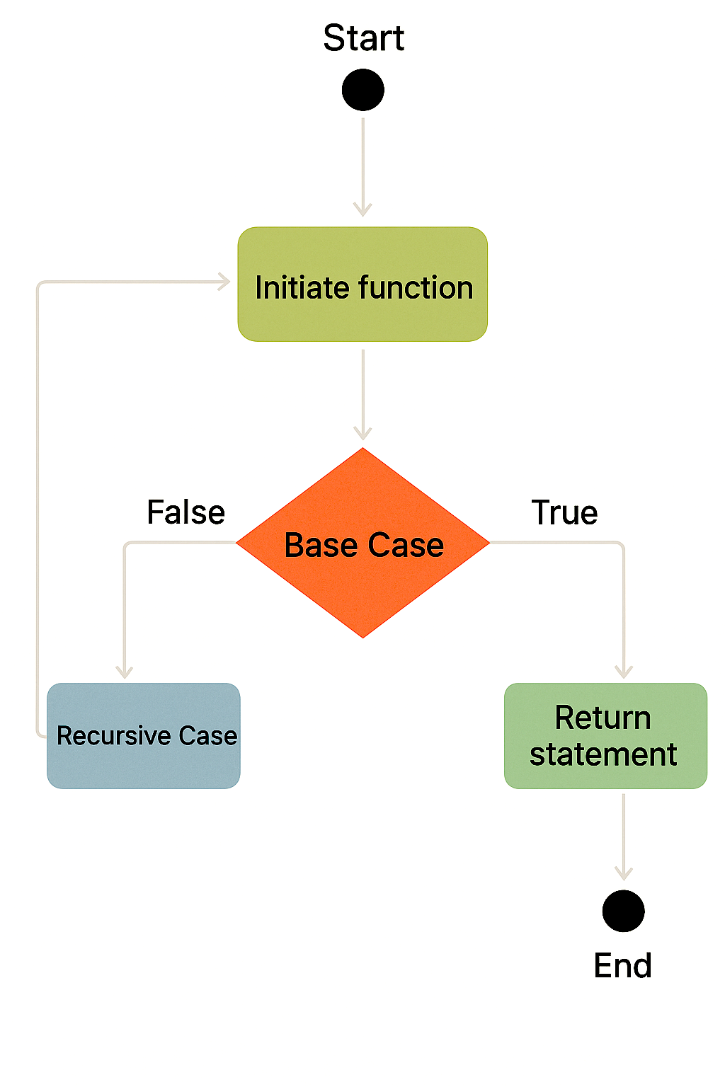
Source: https://betterprogramming.pub/recursive-functions-2b5ce4610c81
Key ingredients
- We want to solve a problem for an input of size $N$
- Inductive reasoning: We can write any case for $N$ in terms of $N - 1$, $N - 2$, etc
- Base cases: the limit of the problem. For example, $0! = 1$, $x_0 = 1$ (initial conditions), etc
Computing the factorial function
We implement two approaches to computing this function: recursion and dynamic programming.
- Problem: Find $N!$
- Inductive reasoning: $N! = N \times (N - 1)!$
- Base case: $0! = 1$
def factorial(n):
    """Compute n factorial via recursion"""
    # print(n, flush=True)
    # Base case
    if n == 0:
        return 1

    # Recursive case in which the function calls itself
    else:
        return n * factorial(n - 1) #+ factorial(n - 2)

factorial(4)
24
### Run a timing test
import timeit
nvals = np.arange(2, 10)
all_times = list()
for n in nvals:
    all_times.append(
        timeit.timeit("factorial(n)", globals=globals(), number=1000000)
    )

plt.figure()
plt.plot(nvals, all_times, 'k')
plt.xlabel('n')
plt.ylabel('Time (s)')
Text(0, 0.5, 'Time (s)')

Instead of recursion, we can instead consider a bottom-up approach to the problem, which starts from the base case and builds up to the desired solution. This is called dynamic programming.
- Problem: Find $N!$
- Inductive reasoning: $N! = N \times (N - 1)!$
- Base case: $0! = 1$
def factorial(n):
    """Compute n factorial, for n >= 0, with dynamic programming."""

    # Start with base case
    if n == 0:
        return 1

    nprev = 1
    for i in range(1, n + 1):
        # print(nprev, flush=True)
        nprev *= i
        # nprev = nprev * i
    return nprev

factorial(4)
1
1
2
6
24
def factorial(n):
    """Compute n factorial, for n >= 0, with dynamic programming."""

    # Start with base case
    if n in [0, 1]:
        return 1

    nprev = 1
    for i in range(2, n + 1):
        nprev *= i
        # nprev = nprev * i
    return nprev


import timeit
nvals = np.arange(2, 15)
all_times = list()
for n in nvals:
    all_times.append(
        timeit.timeit("factorial(n)", globals=globals(), number=1000000)
    )

plt.figure()
plt.plot(nvals, all_times, 'k')
plt.xlabel('n')
plt.ylabel('Time (s)')
Text(0, 0.5, 'Time (s)')

Recursion vs Dynamic programming
Both use a "divide and conquer" approach, but they work in opposite directions
Dynamic programming: start from base cases, and work your way up to $N$
Recursion: start from $N$, then do $N - 1$, etc, until you hit a base case
When working with graphs or trees, we often encounter recursion due to the need to perform depth-first search
When simulating dynamical systems, or processes that don't go backwards, we often run into DP
Dynamic programming is typically $\mathcal{O}(N)$ runtime, $\mathcal{O}(1)$ memory. Recursion is ideally $\mathcal{O}(Log(N))$ runtime, but for the problems we'll see below it's $\mathcal{O}(N)$ runtime, $\mathcal{O}(N)$ memory because we can't skip any steps
A subtlety of timing algorithms
- Why did we only run timing tests for inputs up to $N = 50$? What complicates our analysis if we try timing larger values of $N$?
import timeit
nvals = np.arange(2, 800)
all_times = list()
for n in nvals:
    all_times.append(
        timeit.timeit("factorial(n)", globals=globals(), number=10)
    )

plt.figure()
plt.plot(nvals, all_times, 'k')
[<matplotlib.lines.Line2D at 0x2923c3520>]

It turns out that multiplying large floats has unfavorable scaling with N. Gradeschool is $O(N^2)$ where $N$ is the number of digits, and Karatsuba is $O(N^{1.585})$.
More recursion practice: The Fibonacci sequence
We next apply this approach to computing the Fibonacci sequence, which is famously defined by the recurrence relation
$$\text{Fib}(N) = \text{Fib}(N - 1) + \text{Fib}(N - 2)$$
The first few Fibonacci numbers are $1, 1, 2, 3, 5, 8, 13, 21, 34, 55, \ldots$
def fibonacci(n):
    """Compute the nth Fibonacci number via recursion"""
    # Base cases
    if n == 0:
        return 0
    elif n == 1:
        return 1

    # Recursive case
    else:
        return fibonacci(n - 1) + fibonacci(n - 2)

nvals = np.arange(2, 30)
all_times = list()
for n in nvals:
    all_times.append(
        timeit.timeit("fibonacci(n)", globals=globals(), number=10)
    )

plt.figure(figsize=(9, 6))
plt.semilogy(nvals, all_times)
plt.xlabel("n")
plt.ylabel("Time (s)")
Text(0, 0.5, 'Time (s)')

def fibonacci(n):
    """Compute the nth Fibonacci number via dynamic programming."""

    if n == 0:
        return 0
    elif n == 1:
        return 1

    n1, n2 = 0, 1
    for i in range(2, n + 1):
        n1, n2 = n2, n1 + n2
    return n2


nvals = np.arange(2, 300)
all_times = list()
for n in nvals:
    all_times.append(
        timeit.timeit("fibonacci(n)", globals=globals(), number=1)
    )
plt.plot(nvals, all_times)
[<matplotlib.lines.Line2D at 0x2920dbb20>]

Questions
- Unlike the factorial function, the recursive approach is much slower than the dynamic programming approach, even though they both have the same asymptotic complexity. Why is this?
Recursion versus dynamic programming as discrete-time dynamical systems
We can also think of recursion and dynamic programming as dynamical systems. In this case, the input $N$ is the time variable, and the output is the state of the system at time $N$.
For example, the factorial function can be written as the dynamical system
$$x_{N} = x_{N - 1} \cdot N$$
with initial condition $x_0 = 1$.
The Fibonacci sequence can be written as the dynamical system
$$x_{N} = x_{N - 1} + x_{N - 2}$$
with initial conditions $x_0 = 1$ and $x_1 = 1$.
Dynamic programming corresponds to simulating the dynamical system forward in time, starting from the initial condition. Recursion corresponds to simulating the dynamical system backward in time, starting from the final condition.
Depth-first search versus breadth-first search (solving a maze)
- Generically, recursion vs dynamic programming consists of two different "schema" for solving problems
- In dynamic programming, we start from the base case and work our way up to the solution
- In recursion, we start from big N and then work our way down to the base case
Broadly, we can think of recursion as a "depth-first search" and dynamic programming as a "breadth-first search" of the solution space.
Breadth-first search (BFS) is like dynamic programming

Source: https://www.geeksforgeeks.org/program-for-nth-fibonacci-number/
Depth-first search (DFS) is like recursion
- Worst case: $\mathcal{O}(N_v + N_e)$, where $N_v$, $N_e$ are the number of vertices and edges, respectively
- The number of edges of a hypercube: $N_e = d N_v / 2$, where $d$ is the dimension
- Implies worst-case $\mathcal{O}(N)$ for dfs in square lattice with N vertices

Source: https://www.geeksforgeeks.org/program-for-nth-fibonacci-number/
Looking ahead to Homework 1: The Abelian sandpile
You can implement toppling as either BFS or DFS, or using a purely iterative approach
Physically, what do these different scenarios represent?