Singular Value Decomposition and Image Compression

Preamble: Run the cells below to import the necessary Python packages

This notebook created by William Gilpin. Consult the course website for all content and GitHub repository for raw files and runnable online code.

import numpy as np

# Wipe all outputs from this notebook
from IPython.display import Image, clear_output, display
clear_output(True)

# Import local plotting functions and in-notebook display functions
import matplotlib.pyplot as plt
%matplotlib inline

Eigensystems as dominant "stretching" directions

• Spectral theorem: If a matrix is Hermitian $A^\dagger = A$ (including real-symmetric), then: (1) The eigenvectors are an orthogonal basis, and (2) the eigenvalues are real

• Consistent with our intuition from the dynamical systems view: A "blob" of initial conditions gets anisotropically stretched at different rates along different directions.

• Eigenvalues are invariant to rotations (ie, multiplication by an orthonormal matrix)

Why are Hermitian matrices so important?

Scalar potentials: $$ \dot{\mathbf{x}} = - \nabla U(\mathbf{x}) $$ The "Jacobian" matrix of partial derivatives determines local geometry and concavity, and thus stability and acceleration $$ J_{ij} = \dfrac{\partial \dot{x_i}}{\partial x_j} = - \dfrac{\partial^2 U}{\partial x_i \partial x_j} $$ Dynamical systems (continuous $\dot{\mathbf{x}} = \mathbf{f}(\mathbf{x})$ or discrete $\mathbf{x}_{t} = \mathbf{f}(\mathbf{x}_{t-1})$) always have a Jacobian, but they do not necessarily have a potential.

The loss function or distance matrix when comparing two points $\mathbf{x}, \mathbf{y}$ $$ \mathcal{L}(\mathbf{x}, \mathbf{y}) $$ Has an interaction between two vector components $\mathbf{x}, \mathbf{y}$ $$ \dfrac{\partial \mathcal{L}}{\partial x_i} \dfrac{\partial \mathcal{L}}{\partial y_j} $$

For example, the mean squared error or Euclidean distance, $$ \mathcal{L}(\mathbf{x}, \mathbf{y}) = (\mathbf{x} - \mathbf{y})^T (\mathbf{x} - \mathbf{y}) $$

For example, interactions among pairs of particles with radial forces. In machine learning, $\mathbf{y}$ might be the "true" value of a dataset, and $\mathbf{x}$ might be an approximate value predicted by a model we are training to mimic the data

def random_points_disk(n, r=1):
    """Generate n random points within a disk of radius r"""
    theta = np.random.uniform(0, 2 * np.pi, n)
    r = np.sqrt(np.random.uniform(0, r**2, n)) # notice the sqrt
    x, y = r * np.cos(theta), r *  np.sin(theta)
    return np.vstack((x, y)).T



pts = np.array(random_points_disk(1000))
plt.figure(figsize=(5, 5))
plt.scatter(pts[:,0], pts[:,1])
plt.axis('equal')
plt.title("Points before linear transformation")

# Define a random linear transformation
np.random.seed(0)
A = np.random.uniform(-1, 1, size=(2, 2)) # random 2x2 matrix with entries in [-1, 1]
A = A + A.T # symmetrize matrix to make it Hermitian

# Apply the transformation
pts = pts @ A

plt.figure(figsize=(5,5))
plt.scatter(pts[:,0], pts[:,1])
plt.axis('equal')
plt.title("Points after linear transformation - iteration 1")

# Apply the transformation again
pts = pts @ A

plt.figure(figsize=(5,5))
plt.scatter(pts[:,0], pts[:,1])
plt.axis('equal')
plt.title("Points after linear transformation - iteration 2")

Text(0.5, 1.0, 'Points after linear transformation - iteration 2')

Now let's repeat that iteration many times

pts = np.array(random_points_disk(1000))
all_pts = [np.copy(pts)]
for _ in range(10):
    pts = pts @ A
    all_pts.append(np.copy(pts))

eig_vals, eig_vecs = np.linalg.eig(A)

total_scale = eig_vals[0]**10

plt.figure(figsize=(5,5))
plt.plot(pts[:, 0] / total_scale, pts[:, 1] / total_scale, '.')
plt.axis('equal')

eig_vec1 = eig_vecs[:, 0]
eig_vec2 = eig_vecs[:, 1]
plt.plot([0, eig_vec1[0]], [0, eig_vec1[1]], 'r', lw=2, label="Eigenvector 1")
plt.plot([0, eig_vec2[0]], [0, eig_vec2[1]], 'r', lw=2, label="Eigenvector 2")
plt.legend()
plt.title("Points after many linear transformations, scaled")

Text(0.5, 1.0, 'Points after many linear transformations, scaled')

## Make an interactive video
from ipywidgets import interact, interactive, fixed, interact_manual, Layout
import ipywidgets as widgets

def plotter(i):
    
    total_scale = eig_vals[0]**i
    pts = all_pts[i]

    plt.figure(figsize=(5,5))
    plt.plot(pts[:, 0] / total_scale, pts[:, 1] / total_scale, '.')
    plt.plot([0, eig_vec1[0]], [0, eig_vec1[1]], 'r', lw=2)
    plt.plot([0, eig_vec2[0]], [0, eig_vec2[1]], 'r', lw=2)
    plt.show()

interact(
    plotter, 
    i=widgets.IntSlider(0, 0, 10, 1, layout=Layout(width='800px'))
)

interactive(children=(IntSlider(value=0, description='i', layout=Layout(width='800px'), max=10), Output()), _d…

<function __main__.plotter(i)>

plt.figure(figsize=(8, 6))
plt.plot(np.max(np.array(all_pts) @ eig_vec1, axis=-1), '.r', label="Eigenvector 1")
plt.plot(np.max(np.array(all_pts) @ eig_vec2, axis=-1), '.b', label="Eigenvector 2")
plt.legend()
plt.title("Max span of cloud along eigenvector directions vs. iteration")


plt.plot(np.exp(np.log(eig_vals[0]) * np.arange(11)), color='r', label="Eigenvalue geometric series 1")
plt.plot(np.exp(np.log(-eig_vals[1]) * np.arange(11)), color='b', label="Eigenvalue geometric series 2")
plt.legend()

plt.xlabel("Iteration")
plt.ylabel("Max span")

Text(0, 0.5, 'Max span')

What am I leaving out?

• Non-Hermitian matrices rotate their input space, in addition to anisotopically squeezing it
• • A hot topic of research in stat mech and active matter theory; these describe non-reciprocal interactions (broken detailed balance if the matrix describes kinetics, "odd" elasticity, etc)

What about non-square matrices? Singular Value Decomposition

• $A \in \mathbb R^{N \times M}$.

  • For example, if we have a video of a fluid flow or sensor readings, we might have $N$ frames from $M$ sensors/pixels

• $A$ can be overdetermined ($N > M$) or underdetermined ($N < M$).

• However, we can instead calculate the eigenspectrum of the square matrices $A^\dagger A \in \mathbb R^{M \times M}$ or $A A^\dagger \in \mathbb R^{N \times N}$. We refer to the eigenvectors as the "right" or "left" singular vectors, respectively, and their associated eigenvalues are called the singular values.

  • Note: $A^\dagger A$ and $A A^\dagger$ share the same eigenvalues. Let $\mathbf{x}$ be an eigenvector of $A^\dagger A$ with corresponding eigenvalue $a$: $$A^\dagger A \mathbf{x} = a \mathbf{x} \implies A A^\dagger A \mathbf{x} = a \mathbf{x}$$
  • Consequently, $a$ is also an eigenvalue of $A A^\dagger$ with corresponding eigenvector $A \mathbf{x}$.

• We can now factorize $A$ as: $$ A = U \Sigma V^\dagger $$ where the columns of $U$ are the right singular vectors, the columns of $V$ are the left singular vectors, and $\Sigma$ is a square diagonal matrix. The non-zero entries of $\Sigma$ are the square roots of the non-zero eigenvalues of $A^\dagger A$ or $A A^\dagger$. Since the eigenvalues and eigenvectors can be listed in any order, by convention we normally list the elements in descending order of eigenvalue magnitude.

• Decompose a dataset into characteristic directions in rowspace (left eigenvectors) and characteristic directions in columnspace (right eigenvectors)

• Unlike traditional eigenvalue decomposition, SVD applies to non-square matrices. We can also apply SVD to complex matrices!

• Different interpretations: (1) Geometric, (2) Dynamical, (3) Data compression, pattern discovery

• See image below from Chris Rycroft's AM205 class

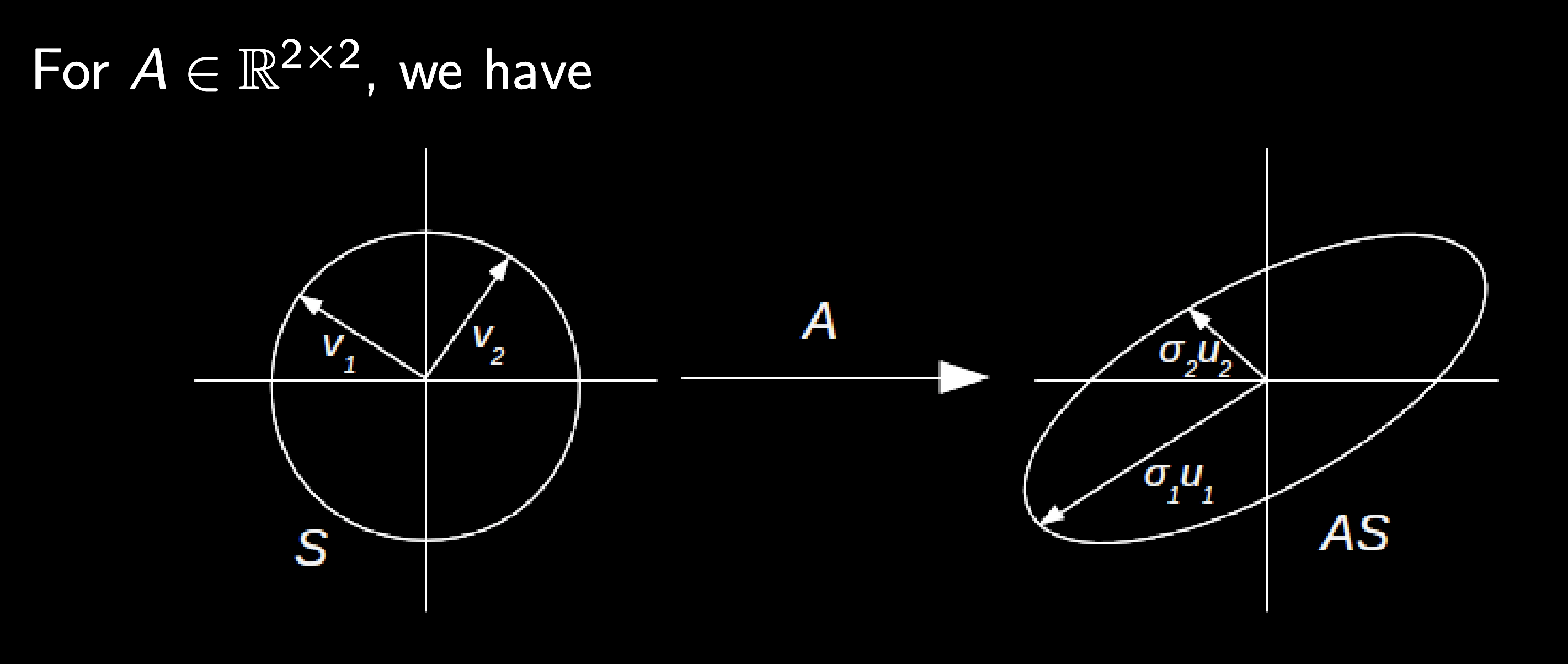
From this diagram, we can define several quantities

• The singular values $\sigma_i$ are the square roots of the eigenvalues of either $A^\dagger A$ or $A A^\dagger$. They are always real and non-negative, and are usually indexed so that they are listed in descending order.

• The left singular vectors $U = \{\mathbf{u}_i\}$ are the eigenvectors of $A^\dagger A$. They are orthogonal unit vectors that point in the directions of the principal axes of $AS$

• The right singular vectors $V = \{\mathbf{v}_i\}$ are the eigenvectors of $A A^\dagger$. They are preimages of the $U$ vectors, so that $A \mathbf{v}_i = \sigma_i \mathbf{u}_i$.

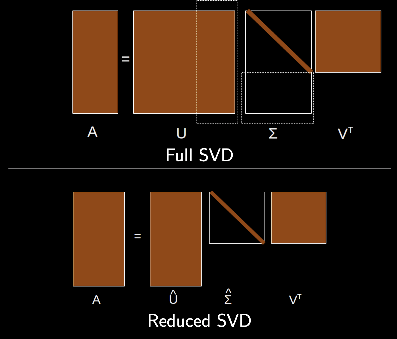
Truncated versus full SVD

• In full SVD, we calculate all $N$ singular values and vectors, and the matrices $U$ and $V$ are square with dimensions $N \times N$ and $M \times M$, respectively, while the matrix $\Sigma$ is rectangular with dimensions $N \times M$.

• In truncated SVD, we calculate only the first $k$ singular values and vectors associated with the largest singular values $\sigma_i$,

• We define the truncated matrices $\tilde U$ of size $N \times k$, $\tilde \Sigma$ of size $k \times k$. $V$ still has size $M \times M$.

• The truncated SVD often approximates the original matrix $A$ well, making it useful for data compression and dimensionality reduction.

$$ A = U \Sigma V^\dagger \approx \tilde U \tilde \Sigma V^\dagger $$

• See image below for a visual representation of the truncated SVD from Chris Rycroft's AM205 class

Dynamical systems interpretation of SVD

In dynamical systems, we might have skew-product structure, where the dynamics of some variables depend only on a subset of the others $$ \begin{cases} x_{t + 1} \!&=& 4 x_t + y_t + 3 z_t \\ y_{t + 1} \!&=& x_t + 2 y_t + 2 z_t \\ z_{t + 1} \!&=& f(z_t, t) \end{cases} $$

Examples: $f(z_t) = z_t + c$ is a a time like variable, $f(z_t) = \eta$ is a random number generator (like we saw for the Ornstein-Uhlenbeck simulation); $f(z_t) = \sin(\omega t)$ is a periodic driver.

Can write this system has rectangular structure $$ \begin{bmatrix} x_{t}\\ y_{t} \end{bmatrix} = \begin{bmatrix} 4 & 1 & 3\\ 1 & 2 & 2 \end{bmatrix} \begin{bmatrix} x_{t}\\ y_{t} \\ z_{t} \end{bmatrix} $$ Our analogy to square matrix dynamics is now a bit more involved, because we can't iterate the system repeatedly without knowing the sequence of $z_t$ values. Notice that if the coupling to the $z$ driver system is zero, then our square "response" subsystem represents an autonomous linear system with Hermitian structure: $x$ affects $y$ as much as $y$ affects $x$/

We can't do any spectral analysis anymore, because our coefficient matrix $A \in \mathbb{R}^{2 \times 3}$. However, we can instead analyze the two square matrices $AA^\dagger \in \mathbb{R}^{2 \times 2}$ and $A^\dagger A \in \mathbb{R}^{3 \times 3}$. This is like analyzing two iterations of a square dynamical system.

a_response = np.array([[4, 1], [1, 2]]).T
print("Two iterations of square response subsystem without driving:")
print(a_response @ a_response.T, end='\n\n')
# print(a_response.T @ a_response, end='\n\n')

# Decoupled limit
a_full = np.array([[4, 1, 0], [1, 2, 0]]).T
print("Left matrix product with zero driving:")
print(a_full @ a_full.T, end='\n\n')
# print(a_full.T @ a_full, end='\n\n')


# Coupled limit
print("Left matrix product with driving:")
a_full = np.array([[4, 1, 3], [1, 2, 2]]).T
print(a_full @ a_full.T, end='\n\n')

Two iterations of square response subsystem without driving:
[[17  6]
 [ 6  5]]

Left matrix product with zero driving:
[[17  6  0]
 [ 6  5  0]
 [ 0  0  0]]

Left matrix product with driving:
[[17  6 14]
 [ 6  5  7]
 [14  7 13]]

Loosely, the left matrix as propagation of an impulse in $z$ across the response subsystem (coupling of dynamical variables to the driver. Tells us about the dependence of response variables on earlier values

a_response = np.array([[4, 1], [1, 2]]).T
print("Two iterations of transpose of square response subsystem without driving:")
print(a_response.T @ a_response, end='\n\n')
# print(a_response.T @ a_response, end='\n\n')


# Decoupled limit
a_full = np.array([[4, 1, 0], [1, 2, 0]]).T
print("Right matrix product with zero driving:")
print(a_full.T @ a_full, end='\n\n')
# print(a_full.T @ a_full, end='\n\n')


# Coupled limit
print("Right matrix product with driving:")
a_full = np.array([[4, 1, 3], [1, 2, 2]]).T
print(a_full.T @ a_full, end='\n\n')

Two iterations of transpose of square response subsystem without driving:
[[17  6]
 [ 6  5]]

Right matrix product with zero driving:
[[17  6]
 [ 6  5]]

Right matrix product with driving:
[[26 12]
 [12  9]]

Loosely, the right matrix tells us about the driver system. If the driver couplings have the form $b = [3, 2]$, then the right matrix is perturbed by elementwise-adding the structured matrix $b b^T$ to the right matrix. The diagonal elements tell us something about how much the different dynamical variables are affected

• This approach might remind you of density matrices

bias = np.array([2, 3])[:, None]
print(bias @ bias.T, end='\n\n')

[[4 6]
 [6 9]]

print(a_full.T @ a_full - a_response.T @ a_response, end='\n\n')

[[9 6]
 [6 4]]

Data representation and compression views

• $A \in \mathbb R^{N \times M}$ is a data matrix, where we have $N$ observations of an $M$ dimensional process. Examples include a video ($N$ is number of frames, $M$ is number of pixels), or a collection of $N$ points in $3D$ space ($M = 3$)
• The left eigenvectors give characteristic "modes" in the data; they have the same dimensionality. The right eigenvectors give us the characteristic "loadings"
• SVD can be used to reduce the dimensionality of a problem by truncating relevant eigenvalues; a basic compression method for high-dimensional data
• The eigenvalue spectrum provides a clue into the dimensionality of the underlying data generating process

Application: Image compression

$$ A = U \Sigma V^\dagger $$

Important: SVD applies to any rectangular matrix. We can reconstruct individual images by treating them as collections of columns, and reconstructing by adding together subsets of characteristic columns

$$ A = \sum_i \sigma_i \mathbf{u}_i \mathbf{v}_i^\dagger $$

If the singular values decay rapidly, then we can approximate the matrix by truncating this sum to the first $k$ terms

from PIL import Image as img

## Local import to open the image
# im = img.open("../resources/hank.png")

## Fetch image from online hosting
import requests
from io import BytesIO
url = "https://raw.githubusercontent.com/williamgilpin/cphy/main/resources/hank.png"
response = requests.get(url)
im = img.open(BytesIO(response.content))

# convert to a numpy image using just the red channel
im = np.array(im)[..., 0]
print("Image shape is", im.shape)
plt.imshow(im, cmap='gray')
plt.axis('off');

Image shape is (372, 248)

# Perform SVD on the image

U, s, V = np.linalg.svd(im)

sigma = s * np.eye(len(s))

# im = U @ sigma @ V.T

# im = U @ np.diag(s) @ V.T
print("U shape is", U.shape)
print("s shape is", s.shape)
print("V shape is", V.shape)

plt.figure(figsize=(8, 5))
plt.semilogy(s)
plt.xlabel("Singular value index");
plt.ylabel("Singular magnitude");
plt.title("Singular values of Hank Hill");

U shape is (372, 372)
s shape is (248,)
V shape is (248, 248)

Us = U[:, :20]
ss = np.diag(s[:20])
Vs = V[:20, :]
print("Us shape is", Us.shape)
print("ss shape is", ss.shape)
print("Vs shape is", Vs.shape)

im_approx = Us @ ss @ Vs
print("Approximation shape is", im_approx.shape)
plt.imshow(im_approx, cmap='gray')
plt.axis('off');

Us shape is (372, 20)
ss shape is (20, 20)
Vs shape is (20, 248)
Approximation shape is (372, 248)

from matplotlib.animation import FuncAnimation
from IPython.display import HTML

# Assuming frames is a numpy array with shape (num_frames, height, width)
# frames = np.array(model.history).copy() 

fig = plt.figure(figsize=(6, 6))
img = plt.imshow(U[:, :1] @ np.diag(s[:1]) @ V[:1, :], vmin=np.min(im), vmax=np.max(im), cmap="gray");
plt.xticks([]); plt.yticks([])
# tight margins
plt.margins(0,0)
plt.gca().xaxis.set_major_locator(plt.NullLocator())

frames = [U[:, :i] @ np.diag(s[:i]) @ V[:i, :] for i in range(1, len(s) + 1)]
def update(frame):
    img.set_array(frame);

ani = FuncAnimation(fig, update, frames=frames, interval=50)
HTML(ani.to_jshtml())

Animation size has reached 20973094 bytes, exceeding the limit of 20971520.0. If you're sure you want a larger animation embedded, set the animation.embed_limit rc parameter to a larger value (in MB). This and further frames will be dropped.

Once Loop Reflect