Numerical Linear algebra and Preconditioning

Preamble: Run the cells below to import the necessary Python packages

This notebook created by William Gilpin. Consult the course website for all content and GitHub repository for raw files and runnable online code.

$$ \newcommand\pmatrix[1]{\begin{pmatrix}#1\end{pmatrix}} \newcommand\bmatrix[1]{\begin{bmatrix}#1\end{bmatrix}} \newcommand\dmatrix[1]{\begin{dmatrix}#1\end{dmatrix}} \renewcommand\vec{\mathbf} $$

## Preamble / required packages
import numpy as np

# Import local plotting functions and in-notebook display functions
import matplotlib.pyplot as plt
from IPython.display import Image, display
%matplotlib inline

Why numerical linear algebra?

• Optimization / machine learning; solving large systems of equations; dynamical systems theory

Two major areas

• Inverting large matrices

• • Linear solving, Conditioning
• • LU Factorization

• Spectral Decomposition

• • Data analysis, dynamical systems
• • QR algorithm

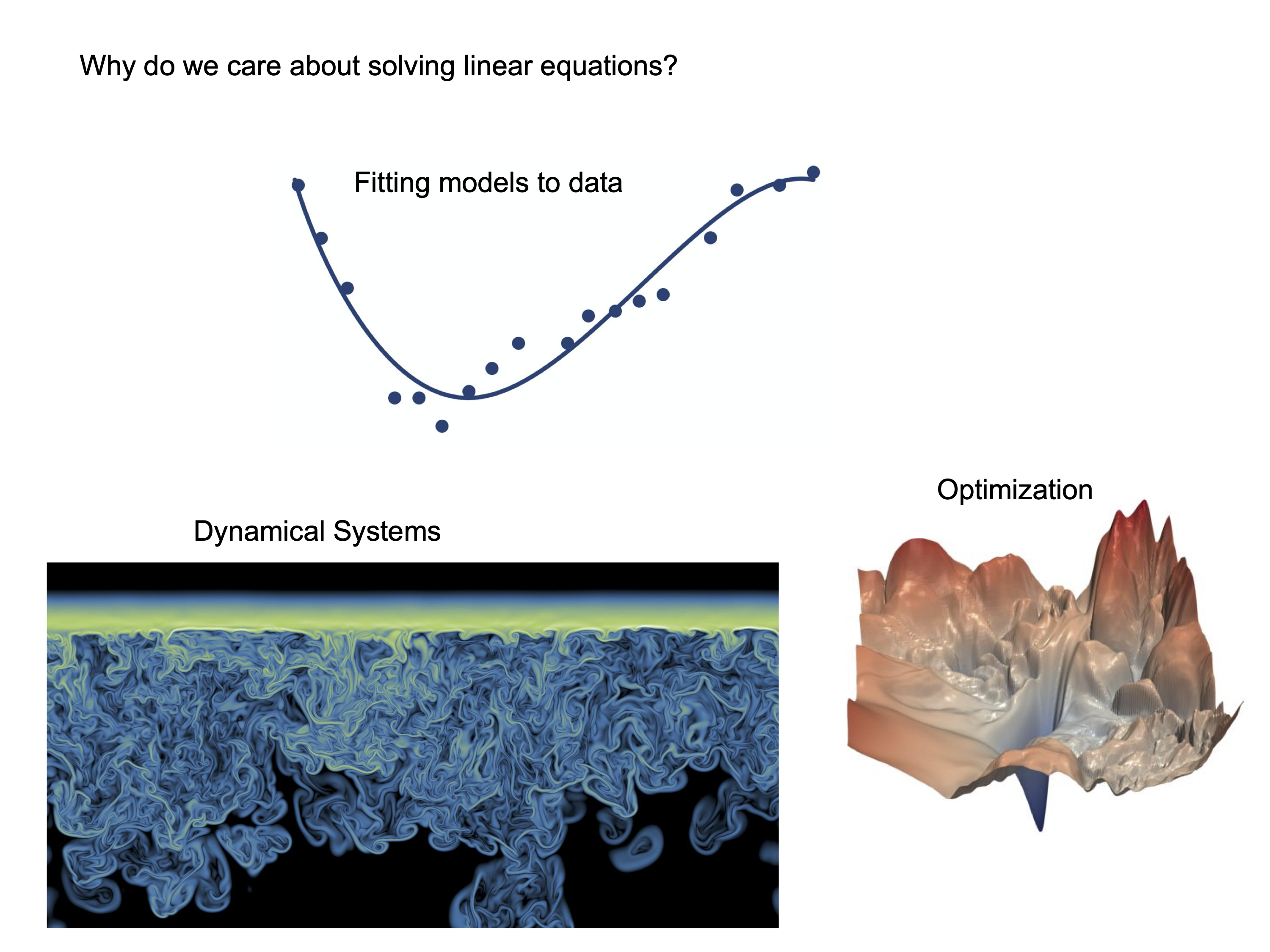
Linear problems

Local constitutive laws give rise to linear matrix equations

• Flow networks, resistivity networks (Ohm's law), Elastic solids (Hooke's law), etc.
• Linear perturbations off stable configurations (eg protein folding)
• $N$ columns denotes the number of particles (atoms, flow nodes, circuit connectsion, etc.)
• $M$ rows denotes the number of equations relating the unknowns
• $M < N$ is underdetermined, $M > N$ is overdetermined. However, this is only true if our matrix has full rank (however, if some variables are functions of others, or some equations are repeated, we can usually eliminate equations or variables to make the problem square)

Write a problem as a linear matrix equation $$ A \mathbf{x} = \mathbf{b} $$

Solve for $\mathbf{x}$ using numerical tools to invert $A$

$$ \mathbf{x} = A^{-1} \mathbf{b} $$

Some issues with finding $A^{-1}$:

• A is too large to store in memory
• A is non-square (over- or under-determined)
• A is singular or very close to singular (two constraint equations are almost, but not quite the same)

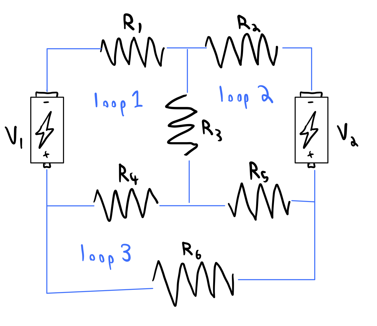
Let $I_i$ denote the current through the $i^{th}$ loop in the circuit, and $V_j$ denote the voltage at the $j^{th}$ node in the circuit. Then, we can write down the following 3 x 3 matrix equation

$$ \begin{bmatrix} R_1 + R_3 + R_4 & R_3 & R_4 \\ R_3 & R_2 + R_3 + R_5 & -R_5 \\ R_4 & -R_5 & R_4 + R_5 + R_6 \end{bmatrix} \begin{bmatrix} I_1 \\ I_2 \\ I_3 \end{bmatrix} = \begin{bmatrix} V_1 \\ V_2 \\ 0 \end{bmatrix} $$

We can now solve for the currents in the circuit using the inverse of the matrix on the left hand side

# Some observed "data"
r1, r2, r3, r4, r5, r6 = np.random.random(6)
v1, v2 = np.random.random(2)


coefficient_matrix = np.array([
    [r1 + r3 + r4, r3, r4], 
    [r3, r2 + r3 + r5,  -r5],
    [r4, -r5, r4 + r5 + r6]
])
voltage_vector = np.array([v1, v2, 0])

# Solve the system of equations
# currents = np.linalg.solve(coefficient_matrix, voltage_vector)
currents = np.linalg.inv(coefficient_matrix) @ voltage_vector
# currents = np.matmul(np.linalg.inv(coefficient_matrix), voltage_vector)
# currents = np.dot(np.linalg.inv(coefficient_matrix), voltage_vector)
# currents = np.einsum("ij,j->i", np.linalg.inv(coefficient_matrix), voltage_vector)
print("Observed currents:", currents)

Observed currents: [ 0.21789554  0.09043251 -0.01222577]

Matrices are collections of vectors

$$ \vec{A} \equiv \pmatrix{\vec{a}_1 & \vec{a}_2 & \cdots & \vec{a}_n} $$

$$ \vec{A} \cdot \vec{x} = \pmatrix{\vec{a}_1 & \vec{a}_2 & \cdots & \vec{a}_n} \pmatrix{x_1 \\ \vdots \\ x_n} = \sum_{k=1}^n x_k \vec{a}_k, $$

• Rank: dimension spanned by column space AND rowspace
• • Implies that if $A \in \mathbb{R}^{M \times N}$, then $\text{rank}(A) \leq \text{min}(M, N)$
• Span: set of points "reachable" by an operator; for linear operators the column psace
• Nullspace: matrices with deficient rank have input spaces that map to zero (think of projection operators)
• Rank-nullity theorem: $dim(Domain) = dim(Image) + dim(NullSpace)$.
• Linear independence among columns implies trivial nullspace, and that input domain dimension matches output image dimensionality/span

Thinking of matrices as dynamical systems

If $A$ is a square matrix, then it can be helpful to think of it as a dynamical system. If not-square, we can always pad zeros.

$\mathbf{x}_{t + 1} = A \mathbf{x}_{t}$

can be written as

$x^i_{t + 1} = \sum_i \mathbf{a}^{(r)} x^i_t$

where $\mathbf{a}^{(r)}$ is a row vector that corresponds to interactions with the other variables that affect the dynamics of $x^i$.

The columnspace dynamics view gives intuition to some properties

• You can't undo a projection: If $A \in \mathbb{R}^{M \times N}$, $B \in \mathbb{R}^{N \times K}$, then $\operatorname {rank} (AB)\leq \min(\operatorname {rank} (A),\operatorname {rank} (B)).$
• For a dynamical system, this means that if you have a system that is evolving in a lower dimensional space, you can't recover the original state from the lower dimensional state.

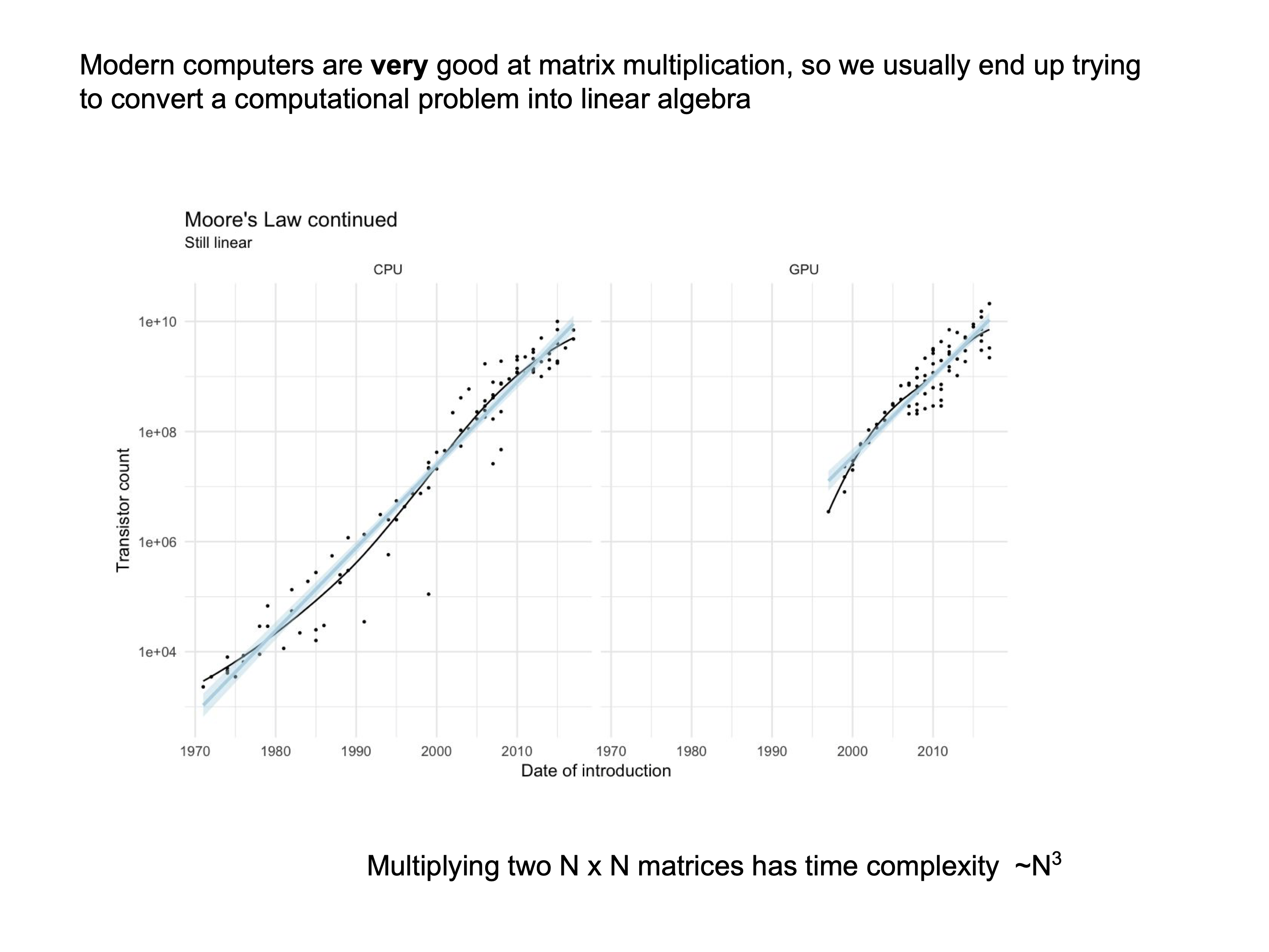
Consider the time complexity of matrix inversion

Given $A \in \mathbb{R}^{M \times N}$ and $\mathbf{b} \in \mathbb{R}^{N}$, we wish to solve $A \mathbf{x} = \mathbf{b}$

• Best case scenario: $A$ is a diagonal matrix

import numpy as np
diag_vals = np.random.randn(5)
ident = np.identity(5)
a = ident * diag_vals
plt.figure(figsize=(3,3))
plt.imshow(a, vmin=-1, vmax=1)

# # ## Create inverse directly
ident = np.identity(5)
ainv = ident * (1 / diag_vals)
plt.figure(figsize=(3,3))
plt.imshow(ainv, vmin=-1, vmax=1)


plt.figure(figsize=(3,3))
plt.imshow(a @ ainv, vmin=-1, vmax=1)

<matplotlib.image.AxesImage at 0x2b6ee5850>

$A^{-1} A = I$

We can see that the time complexity of solving this problem is $O(N)$, because just have to touch each diagonal element once, to invert it.

Inverting an upper-triangular matrix

$$ \begin{bmatrix} a_{11} & a_{12} & a_{13} & \cdots & a_{1N} \\ 0 & a_{22} & a_{23} & \cdots & a_{2N} \\ 0 & 0 & a_{33} & \cdots & a_{3N} \\ \vdots & \vdots & \vdots & \ddots & \vdots \\ 0 & 0 & 0 & \cdots & a_{NN} \\ \end{bmatrix} $$

Key: remember that inverting this matrix is equivalent to solving a system of equations

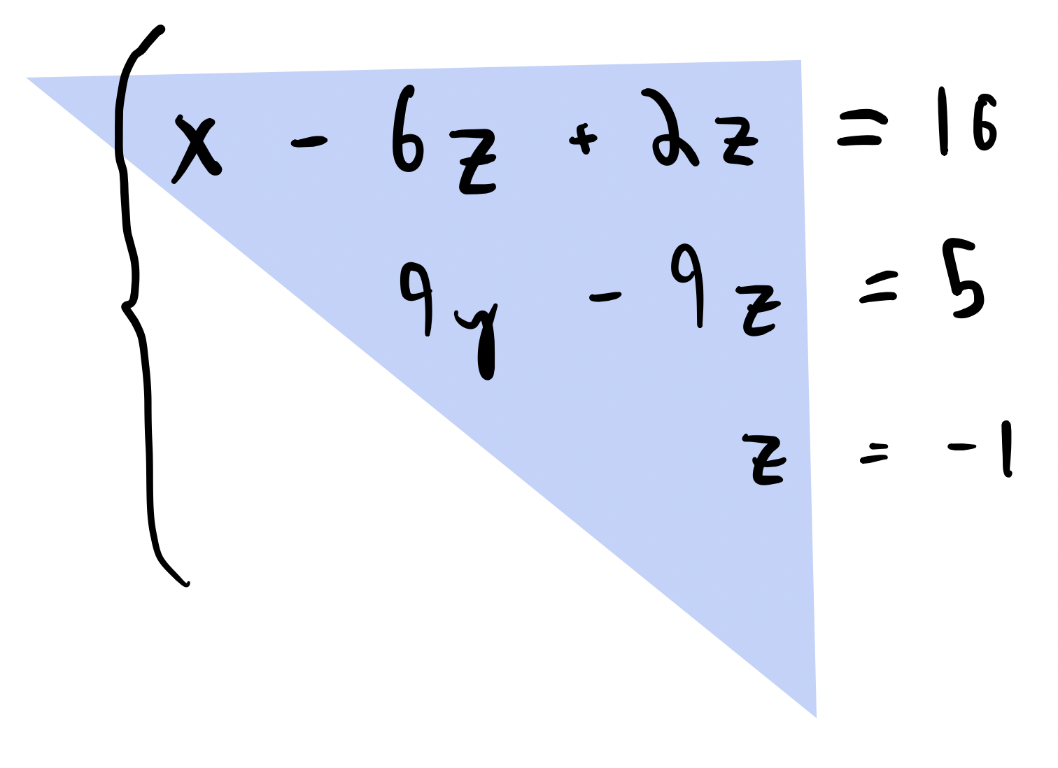
• Heuristic: Solve the easy equation, and work your way up by substituting back into previous equations
• If we count out these operations, they are equivalent to $\sim\mathcal{O}(N^2)$

What about inversion of a full $N \times N$ matrix?

Naive inversion: schoolyard algebra (Gauss-Jordan)

$$ A = {\displaystyle {\begin{bmatrix}1&3&1\\1&1&-1\\3&11&6\end{bmatrix}}}, \text{\quad} \mathbf{b} = {\begin{bmatrix}9\\1\\35\end{bmatrix}} $$ Can reduce by multiply by constants or adding two rows. For example, we subtract row 1 from row 2 in the first step $$ {\displaystyle {\begin{bmatrix}1&3&1&9\\1&1&-1&1\\3&11&6&35\end{bmatrix}}\to {\begin{bmatrix}1&3&1&9\\0&-2&-2&-8\\3&11&6&35\end{bmatrix}}\to {\begin{bmatrix}1&3&1&9\\0&-2&-2&-8\\0&2&3&8\end{bmatrix}}\to {\begin{bmatrix}1&3&1&9\\0&-2&-2&-8\\0&0&1&0\end{bmatrix}} } $$

We can write the Gauss-Jordan algorithm as a matrix multiplication $$ \begin{bmatrix}1&3&1\\1&1&-1\\3&11&6\end{bmatrix} \begin{bmatrix}1&0&0\\-1&1&0\\0&-1&1\end{bmatrix} = \begin{bmatrix}1&0&0\\0&1&0\\0&0&1\end{bmatrix} $$

Based on this, can we guess the time complexity of Gauss-Jordan elimination?

Sensitivity of matrix inversion: The condition number

• Tells us how difficult a matrix will be to invert
• A measure of how sensitive a matrix is to small perturbations
• The condition number of a matrix is the ratio of the largest singular value to the smallest singular value
• Matrix norm: $|| A ||_p = (\sum_{ij} |a_{ij}|^p)^{1/p}$. The familiar Frobenius norm is $p=2$ in this equation
• Condition number: $\kappa \equiv || A ||_p || A^{-1} ||_p$

def matrix_norm(A, p=2):
    """Compute the p-norm of a matrix A."""
    return np.sum(np.abs(A)**p)**(1/p)

def condition_number(A, p=2):
    """Compute the condition number of a matrix A"""
    return matrix_norm(A, p) * matrix_norm(np.linalg.inv(A), p)

• This next block of code creates an $N \times N$ matrix that initially corresponds to a matrix whose columns are all identical column vectors, $\mathbf{a}_1$.

• We then add an $N \times N$ matrix of random numbers drawn from the unit normal distribution, with mean $0$ and standard deviation $\epsilon$

$A = [\mathbf{a}_1\;\; \mathbf{a}_1 \;\;\mathbf{a}_1\;\; \mathbf{a}_1] + \epsilon E$

$ E \in \mathbb{R}^{N \times N}$

$ E_{ij} \sim \mathcal{N}(0, 1)$

a1 = np.random.random(4)

noise_levels = np.logspace(-5, 3, 500)
all_condition_numbers = []
for noise_level in noise_levels:
    a = np.vstack(
        [
            a1 + np.random.normal(size=a1.shape) * noise_level, 
            a1 + np.random.normal(size=a1.shape) * noise_level, 
            a1 + np.random.normal(size=a1.shape) * noise_level, 
            a1 + np.random.normal(size=a1.shape) * noise_level
        ]
    )
    all_condition_numbers.append(condition_number(a))

plt.figure(figsize=(8, 6))
plt.loglog(noise_levels, all_condition_numbers)
plt.xlabel("Column disalignment noise")
plt.ylabel("Condition number")

Text(0, 0.5, 'Condition number')

## Make an interactive video
from ipywidgets import interact, interactive, fixed, interact_manual, Layout
import ipywidgets as widgets

# ## Find fixed axis bounds
# vmax = np.max(np.array(eq.history), axis=(0, 1))
# vmin = np.min(np.array(eq.history), axis=(0, 1))

eps = np.logspace(-5, 0, 100)
def plotter(i):
    # plt.close()
    a_ill = np.array([
        [1, 1], 
        [1, 1 + eps[i]], 
    ])
    plt.figure()
    plt.arrow(0, 0, *a_ill[0], head_width=0.05, head_length=0.1, color='black')
    plt.arrow(0, 0, *a_ill[1], head_width=0.05, head_length=0.1, color='b')
    plt.xlim(0, 2)
    plt.ylim(0, 2)
    # annotate condition number on plot
    plt.annotate(
        f"Condition number: {condition_number(a_ill):.2f}",
        xy=(0.5, 1.5),
        xytext=(0.5, 1.5),
        fontsize=16
    )
    plt.show()

interact(
    plotter, 
    i=widgets.IntSlider(0, 0, len(eps) - 1, 1, layout=Layout(width='800px'))
)

interactive(children=(IntSlider(value=0, description='i', layout=Layout(width='800px'), max=99), Output()), _d…

<function __main__.plotter(i)>

Practical implications of ill-conditioned matrices

import time
import matplotlib.pyplot as plt


sizes = np.arange(100, 2000, 10)
condition_numbers = []
times = []
for n in sizes:
    # Generate a random matrix and a random vector
    A = np.random.rand(n, n)
    b = np.random.rand(n)
    
    # Compute the condition number
    cond_num = np.linalg.cond(A)

    # Measure the time to solve the system
    start_time = time.time()
    np.linalg.solve(A, b)
    end_time = time.time()
    
    # Store the time taken and condition number
    condition_numbers.append(cond_num)
    times.append(end_time - start_time)

plt.figure()
plt.loglog(condition_numbers, times, '.', markersize=10)
plt.xlabel('Condition Number')
plt.ylabel('Time Taken (s)')
plt.title('Condition Number vs Time Taken')
plt.show()

We can always think of matrices in terms of dynamical systems

• Below, we thing of a 2 x 2 matrix as a dynamical system acting on points in the plane

• We initialize a random point in the plane, and then initialize a second point a very small distance away from the first point

• We apply the matrix to both points for many timesteps, and we record the distance between the two points at each timestep

a_good = np.array([
    [1, 1], 
    [1, 1 + 1e0], 
])

a_ill = np.array([
    [1, 1], 
    [1, 1 + 1e-14], 
])

np.linalg.cond(a_good), np.linalg.cond(a_ill)

(6.854101966249685, 393638158031468.2)

initial_condition = np.array([1, 1])
initial_condition_perturbed = initial_condition + 1e-5

# repeatedly apply the matrix to the initial condition and another one super close to it
all_points = [np.array([initial_condition, initial_condition_perturbed])]
for i in range(100):
    all_points.append(a_good @ all_points[-1].T)
# Calculate separation between the two points vs time
pairwise_dispersion = np.linalg.norm(np.diff(np.array(all_points), axis=1), axis=(1, 2))
plt.figure(figsize=(8, 6))
plt.semilogy(pairwise_dispersion)
plt.xlabel("Time step")
plt.ylabel("Distance between points")

# # repeatedly apply the matrix to the initial condition and another one super close to it
all_points = [np.array([initial_condition, initial_condition_perturbed])]
for i in range(100):
    all_points.append(a_ill @ all_points[-1].T)
# Calculate separation between the two points vs time
pairwise_dispersion = np.linalg.norm(np.diff(np.array(all_points), axis=1), axis=(1, 2))
plt.semilogy(pairwise_dispersion)
plt.xlabel("Time step")
plt.ylabel("Distance between points")
plt.legend(["Ill-conditioned", "Well-conditioned"])

<matplotlib.legend.Legend at 0x2b7d31ed0>

• Notice how the spacing between the two points grows exponentially with time, but it grows more slowly under the action of the ill-conditioned matrix

• Conceptually, the ill-conditioned matrix acts as if the two points are confined to a lower-dimensional space. Generically, the ill-conditioning is associated with a slow manifold in the dynamics

What about the inverse of a matrix?

• We can think of the inverse of a matrix as inverting the dynamics in time

ainv_ill = np.linalg.inv(a_ill)
ainv_good = np.linalg.inv(a_good)

initial_condition = np.array([1, 1])
initial_condition_perturbed = initial_condition + 1e-5

# repeatedly apply the matrix to the initial condition and another one super close to it
all_points = [np.array([initial_condition, initial_condition_perturbed])]
for i in range(100):
    all_points.append(ainv_ill @ all_points[-1].T)
# Calculate separation between the two points vs time
pairwise_dispersion = np.linalg.norm(np.diff(np.array(all_points), axis=1), axis=(1, 2))
plt.figure(figsize=(8, 6))
plt.semilogy(pairwise_dispersion)
plt.xlabel("Time step")
plt.ylabel("Distance between points")

# repeatedly apply the matrix to the initial condition and another one super close to it
all_points = [np.array([initial_condition, initial_condition_perturbed])]
for i in range(100):
    all_points.append(ainv_good @ all_points[-1].T)
# Calculate separation between the two points vs time
pairwise_dispersion = np.linalg.norm(np.diff(np.array(all_points), axis=1), axis=(1, 2))
plt.semilogy(pairwise_dispersion)
plt.xlabel("Time step")
plt.ylabel("Distance between points")
plt.legend(["Ill-conditioned", "Well-conditioned"])

/var/folders/xt/9wdl4pmx26gf_qytq8_d528c0000gq/T/ipykernel_23556/3318648983.py:10: RuntimeWarning: overflow encountered in matmul
  all_points.append(ainv_ill @ all_points[-1].T)

<matplotlib.legend.Legend at 0x16d5b9ed0>

• We can see that the inverse of the ill-conditioned matrix is much more sensitive to small perturbations in the input space

• Why does this matter? Recall our least squares problem

$$ \mathbf{x} = A^{-1} \mathbf{b} $$

• If $A$ is ill-conditioned, then small perturbations in $\mathbf{b}$ can lead to large perturbations in $\mathbf{x}$

Interpretation of ill-conditioning in physical systems

• Ohm's law: $I = R^{-1} V$. Any small fluctuations in the voltage at a set of nodes can lead to large fluctuations in the currents

• Elasticity: $X = K^{-1} F$. Small perturbations in the applied forces can lead to large fluctuations in the displacements

The curse of dimensionality

• We will perform a numerical experiment to see how the condition number of a matrix scales with the dimensionality of the matrix.

• We will generate a series of random matrices of varying dimensionality, and compute the condition number of each matrix.

a1 = np.random.random(4)

all_condition_numbers = []
all_norms = []
nvals = np.arange(3, 600)
for n in nvals:
    a = np.random.normal(size=(n, n))
    a /= n**2 ## Sanity check that we aren't getting naive scaling
    all_condition_numbers.append(np.linalg.cond(a))
    all_norms.append(matrix_norm(a))
plt.figure(figsize=(8, 6))
plt.loglog(nvals, all_condition_numbers)
# plt.loglog(nvals, nvals)
plt.xlabel("Matrix size")
plt.ylabel("Condition number")

Text(0, 0.5, 'Condition number')

• Generically, a random matrix has a condition number that scales as $\kappa \sim \mathcal{O}(N)$

plt.figure(figsize=(8, 6))
plt.loglog(nvals, all_condition_numbers)
plt.loglog(nvals, 2*nvals**(1), '--')
plt.xlabel("Matrix size")
plt.ylabel("Condition number")

Text(0, 0.5, 'Condition number')

Concentration of measure

• Random high-dimensional vectors tend to be nearly orthogonal

• The code below calculates random Gaussian vectors with zero mean and unit variance in $N$ dimensions, and then calculates the angle between them

a1, a2 = np.random.randn(10), np.random.randn(10)
a1, a2 = a1 / np.linalg.norm(a1), a2 / np.linalg.norm(a2) # Convert to unit vectors
print(np.dot(a1, a2))

a1, a2 = np.random.randn(10000), np.random.randn(10000)
a1, a2 = a1 / np.linalg.norm(a1), a2 / np.linalg.norm(a2) # Convert to unit vectors
print(np.arccos(np.dot(a1, a2)))

0.49886931686533487
-0.012629821259598873

nvals = np.arange(3, 500)

all_angs = []
all_errs = []
for n in range(3, 500):

    # average across 100 replicates
    all_replicates = []
    for _ in range(400):
        a1 = np.random.randn(n)
        a2 = np.random.randn(n)
        ang = np.arccos(np.dot(a1, a2) / (np.linalg.norm(a1) * np.linalg.norm(a2)))
        all_replicates.append(np.abs(ang)) # abs because of negative angles
    all_angs.append(np.mean(all_replicates))
    all_errs.append(np.std(all_replicates))

print(f"Estimate of asymptotic value: {all_angs[-1]:.2f} +/- {all_errs[-1]:.2f}")

plt.figure(figsize=(8, 6))
plt.semilogx(nvals, all_angs)
plt.fill_between(nvals, np.array(all_angs) - np.array(all_errs), np.array(all_angs) + np.array(all_errs), alpha=0.5)
plt.xlabel("Dimensionality")
plt.ylabel("Angle between random vectors")

Estimate of asymptotic value: 1.58 +/- 0.05

Text(0, 0.5, 'Angle between random vectors')

The birthday paradox: A loose argument why large, random square matrices tend to be ill-conditioned

A matrix will be ill-conditioned in any pair of columns is close to collinear. Imagine a universe where every randomly-sampled vector is a unit vector with exactly one nonzero element. What is the probability that a matrix comprising a set of $N$ length-$N$ unit vectors are mutually orthogonal?

def sample_unit(n):
    a = np.random.randn(n)
    a0 = np.zeros(n)
    a0[np.argmax(a)] = 1
    return a0

sample_unit(10)

array([0., 0., 0., 0., 0., 0., 1., 0., 0., 0.])

n_repeats = 500
nvals = np.arange(3, 300)
all_products_vals = []
for n in nvals:
    products = [sample_unit(n) @ sample_unit(n) for _ in range(n_repeats)]
    all_products_vals.append(np.mean(products))

plt.figure(figsize=(6, 6))
plt.loglog(nvals, all_products_vals)
# plt.loglog(nvals, 1 / nvals, '--')
plt.xlabel("Dimensionality")
plt.ylabel("Mean dot product")

Text(0, 0.5, 'Mean dot product')

Given just two vectors of length $N$, the probability of mutual orthogonality is $$ P_{ortho} = \bigg(1\bigg) \bigg(\dfrac{N -1}{N}\bigg) = \bigg(\dfrac{N}{N}\bigg) \bigg(\dfrac{N -1}{N}\bigg) $$ As $N \to \infty$, the probability of two vectors being orthogonal goes to zero as $\sim\mathcal{O}(1/N)$

Now, given $N$ vectors, the probability of mutual orthogonality is $$ P_{ortho} =\dfrac{N!}{N^N} $$

Stirling's approximation: at large $N$, $N! \sim {\sqrt {2\pi N}}\left({\frac {N}{e}}\right)^{N}$ $$ P_{ortho} \sim \sqrt{2\pi N}e^{-N} $$

The exponential term dominates at large $N$, and so the odds of getting lucky and having an invertible matrix vanish exponentially with $N$. In this case, the condition number diverges towards infinity.

For random continuous matrices, large matrices have a vanishing probability of being truly singular (you never draw the same multivariate sample twice), but their condition number grows quickly making them "softly" singular

nvals = np.arange(3, 100)
plt.loglog(nvals, 1 - np.sqrt(2 * np.pi * nvals) * np.exp(-nvals))
plt.title("Probability of a random permutation matrix being ill-conditioned")
plt.xlabel("Matrix size")
plt.ylabel("Probability")

Text(0, 0.5, 'Probability')

The Johnson–Lindenstrauss lemma

• A small set of points in a high-dimensional space can be embedded into a space of much lower dimension in such a way that distances between the points are nearly preserved

• We can use random projections to reduce the dimensionality of a matrix, and then solve the problem in the lower-dimensional space

import numpy as np
import matplotlib.pyplot as plt

# Generate a set of high-dimensional vectors (e.g., 1000-dimensional)
num_points = 30
dim = 4000
X = np.random.rand(num_points, dim)

# Define the reduced dimension and epsilon
new_dim = 500  # You can vary this based on the lemma's guidelines for your chosen epsilon
epsilon = 0.5

# Create a random projection matrix
projection_matrix = np.random.randn(new_dim, dim) / np.sqrt(new_dim)

# Project the high-dimensional vectors into the lower-dimensional space
X_new = X.dot(projection_matrix.T)

# Compute pairwise distances in the original and reduced spaces
dist_original = np.linalg.norm(X[:, None, :] - X[None, :, :], axis=-1)
dist_new = np.linalg.norm(X_new[:, None, :] - X_new[None, :, :], axis=-1)

# Step 6: Plot the original and new distances
plt.figure(figsize=(10, 5))

plt.subplot(1, 2, 1)
plt.imshow(dist_original, origin='lower', vmin=np.min(dist_original), vmax=np.max(dist_original))
plt.title('Original Distances')
plt.colorbar()

plt.subplot(1, 2, 2)
plt.imshow(dist_new,  origin='lower', vmin=np.min(dist_original), vmax=np.max(dist_original))
plt.title('New Distances')
plt.colorbar()
plt.tight_layout()
plt.show()


# Check that the distances are approximately preserved to within epsilon
print(np.all((1 - epsilon) * dist_original <= dist_new))
print(np.all(dist_new <= (1 + epsilon) * dist_original))

True
True

Condition number and the irreversibility of chaos

The Lorenz equations are a set of three coupled nonlinear ordinary differential equations that exhibit a transition to chaos,

$$ \begin{aligned} \dot{x} &= \sigma (y-x) \\ \dot{y} &= x (\rho - z) - y \\ \dot{z} &= x y - \beta z \end{aligned} $$

where $\sigma$, $\rho$, and $\beta$ are parameters. These equations exhibit chaotic dynamics when $\sigma = 10$, $\rho = 28$, and $\beta = 8/3$. The degree of chaos can be varied by changing the parameter $\rho$.

We can linearize these equations by computing the Jacobian matrix, which is the matrix of all first-order partial derivatives of the system. The Jacobian matrix is

$$ \mathbb{J}(\mathbf{x}) = \dfrac{d \mathbf{\dot{x}}}{d \mathbf{x}} = \begin{bmatrix} -\sigma & \sigma & 0 \\ \rho - z & -1 & -x \\ y & x & -\beta \end{bmatrix} $$

Notice how, unlike a globally linear dynamical system, the Jacobian matrix $\mathbb{J}(\mathbf{x})$ is a function of the state vector $\mathbf{x}$. This means that the linearization of the system is only valid for a small region of state space around the point $\mathbf{x}$.

We can use the linearization of this system to create a simple finite-differences integration scheme. The linearized system is

$$ \mathbf{x}_{t+1} = \mathbf{x}_t + \Delta t\, \mathbb{J}(\mathbf{x}_t) \mathbf{x}_t $$

or, equivalently,

$$ \mathbf{x}_{t+1} = \left( \mathbb{I} + \Delta t\, \mathbb{J}(\mathbf{x}_t) \right) \mathbf{x}_t $$

where $\mathbb{I}$ is the identity matrix.

We will see more sophisticated integration schemes later in the course, but this particular update rule in this case is a linear scheme with a forward update rule.

class Lorenz:
    """
    The Lorenz equations describe a chaotic system of differential equations.
    """
    def __init__(self, sigma=10, rho=28, beta=8/3):
        self.sigma = sigma
        self.rho = rho
        self.beta = beta

    def rhs(self, X):
        """Returns the right-hand side (vector time derivative) of the Lorenz equations."""
        x, y, z = X # Argument unpacking
        return np.array([
            self.sigma * (y - x), 
            x * (self.rho - z) - y, 
            x * y - self.beta * z
        ])
    
    def jacobian(self, X):
        """Returns the Jacobian of the Lorenz equations."""
        x, y, z = X
        return np.array([
            [-self.sigma, self.sigma, 0], 
            [self.rho - z, -1, -x], 
            [y, x, -self.beta]
        ])
    
    def integrate(self, x0, t0, t1, dt):
        """
        Integrate using the jacobian and forward euler
        """
        x = x0
        all_x = [x]
        all_t = [t0]
        while t0 < t1:
            jac = self.jacobian(x) # because it's nonlinear we need to recompute at each step
            x += jac @ x * dt
            t0 += dt
            all_x.append(x.copy())
            all_t.append(t0)
        return np.array(all_x), np.array(all_t)
    


# A parameter value that doesn't exhibit chaos
eq = Lorenz(rho=10)
x0 = np.array([2.44948974, 2.44948974, 4.5]) 
x_nonchaotic, all_t = eq.integrate(x0, 0., 100., 0.01)
plt.figure()
plt.plot(x_nonchaotic[:, 0], x_nonchaotic[:, 2])

# # A parameter value that exhibits chaos
eq = Lorenz()
x0 = np.array([-5.0,  -5.0, 14.4]) # pick initial condition on the attractor
x_chaotic, all_t = eq.integrate(x0, 0., 100., 0.01)
plt.figure()
plt.plot(x_chaotic[:, 0], x_chaotic[:, 2])

[<matplotlib.lines.Line2D at 0x2d5c15990>]

The condition number

Now we can evaluate the condition number of the Jacobian matrix $\mathbb{J}(\mathbf{x})$ at a particular point $\mathbf{x}$. The condition number is defined as

$$ \kappa(\mathbf{x}) = || \mathbb{J}(\mathbf{x}) || \, || \mathbb{J}^{-1}(\mathbf{x}) || $$

Because the system is not Hamiltonian, we cannot simplify this expression using the eigenvalues of the Jacobian matrix.

jac_chaotic = np.array([eq.jacobian(x) for x in x_chaotic])
plt.figure(figsize=(8, 4))
plt.semilogy(
    [np.linalg.cond(item) for item in jac_chaotic]
)
plt.xlabel("Time step")
plt.ylabel("Condition number")

# plt.figure(figsize=(8, 4))
# plt.plot(
#     x_chaotic[:, 0]
# )
# plt.xlabel("Time step")
# plt.ylabel("x(t)")

## Why???
# plt.figure(figsize=(6, 6))
# plt.scatter(
#     x_chaotic[:, 0], x_chaotic[:, 2], c=[np.log10(np.linalg.cond(item)) for item in jac_chaotic]
# )
# plt.xlabel("x(t)")
# plt.ylabel("y(t)")

jac_nonchaotic = np.array([eq.jacobian(x) for x in x_nonchaotic])
plt.figure(figsize=(8, 4))
plt.semilogy(
    [np.linalg.cond(item) for item in jac_nonchaotic[:]]
)
plt.xlabel("Time step")
plt.ylabel("Condition number")

Text(0, 0.5, 'Condition number')

Questions

• In the nonchaotic case, why is the condition number still a positive, albeit smaller, number? What physical circumstances might decrease this number?

• In higher dimensioins, it's easier to become ill-conditioned

• In higher dimenisons there are more route to chaos

Preconditioning

• Use domain or problem knowledge to transform a matrix into a better-conditioned problem
• Depends strongly on the problem type, and any known structure in the matrix we seek to invert
• In ML, using domain knowledge to restrict model space is known as an "inductive bias"

For example, for a linear problem we might seek the "left" preconditioning matrix $Q$ $$ A \mathbf{x} = \mathbf{y} \\ Q A \mathbf{x} = Q \mathbf{y} \\ \mathbf{x} = (Q A)^{-1} Q \mathbf{y} \\ $$ Hopefully, $(Q A)^{-1}$ is easier to compute than $A^{-1}$

## Make a high condition number matrix
a1 = np.random.random(4)
a = np.vstack([a1, a1, a1, a1]) 
a += np.random.random(a.shape) * 1e-5
print("Full condition number:", condition_number(a), "\n")

## partial condition number
q = 1 / a1 * np.eye(4)

print("Condition number of Q:", condition_number(q @ a.T), "\n")

Full condition number: 3905287.6462541786 

Condition number of Q: 4679089.951615427 

Jacobi preconditioning

Another option is to perform the preconditioning in a different order $$ A \mathbf{x} = \mathbf{y} \\ A P^{-1} P \mathbf{x} = \mathbf{y} \\ $$ where we first solve for a latent variable $\mathbf{z}$ $$ \mathbf{z} = (A P^{{-1}})^{-1} \mathbf{y} $$ And then separately solve for the unknown $\mathbf{x}$ $$ \mathbf{x} = P^{-1} \mathbf{z} $$

There are many heuristics for choosing $Q$ or $P$ depending on the problem. Some common ones are listed here. Conceptually, one of the simplest approaches is Jacobi preconditioning, where we choose $P$ to be a diagonal matrix with the same diagonal elements as $A$.

$$ P = \text{diag}(A) $$

$$ P^{-1} = \text{diag}(A)^{-1} $$

Recall that inverting a diagonal matrix only takes $\mathcal{O}(N)$ time, because we only have to invert each diagonal element. This is much faster than the $\mathcal{O}(N^3)$ time required to invert a general matrix.

The concept of preconditioning motivates change of basis and spectral methods for solving partial differential equations---even though many integral transforms are information-preserving and thus equivalent to a change of basis, they can be used to transform a problem into a better-conditioned form.

## Make a high condition number matrix
a1 = np.random.random(4)
a = np.vstack([a1, a1, a1, a1]) 
a += np.random.random(a.shape) * 1e-5
print("Full condition number:", condition_number(a), "\n")

# This is called Jacobi conditioning
p = np.identity(a.shape[0]) * np.diag(a)
pinv = np.identity(a.shape[0]) * 1 / np.diag(a) # Inverse of diagonal matrix easy to calculate

print("Partial condition number 1: ", condition_number(a @ pinv))
print("Partial condition number 2: ", condition_number(p))

Full condition number: 3479763.5582248624 

Partial condition number 1:  3055250.443096764
Partial condition number 2:  4.479215399524707

How much does the condition number affect matrix inversion in practice?

• We will generate a large number of random matrices of varying condition number, and then solve the matrix inversion problem for each matrix

• We will use numpy's built-in matrix inversion routine to solve the problem

• We will measure the time it takes to solve the problem for each matrix

n_trials = 100
time_without_precond = []
time_with_precond = []
for _ in range(n_trials):
    # Generate a random matrix and a random vector
    A = np.random.rand(4000, 4000)
    b = np.random.rand(4000)

    # Measure the time to solve the system
    start_time = time.time()
    sol = np.linalg.solve(A, b)
    # Ainv = np.linalg.inv(A)
    # sol = Ainv @ b
    end_time = time.time()
    time_taken = end_time - start_time
    time_without_precond.append(time_taken)

    # Now let's try preconditioning
    P = np.identity(A.shape[0]) * 1 / np.diag(A)
    start_time = time.time()
    A_precond = P @ A
    b_precond = P @ b
    sol = np.linalg.solve(A_precond, b_precond)
    end_time = time.time()
    time_taken = end_time - start_time
    time_with_precond.append(time_taken)

plt.figure(figsize=(8, 8))
plt.plot(time_without_precond, time_with_precond, '.')
plt.plot(np.sort(time_without_precond), np.sort(time_without_precond), '--k', label="Equal runtime")
# plt.xlim(np.min(time_without_precond), np.max(time_without_precond))
# plt.ylim(np.min(time_without_precond), np.max(time_without_precond))
plt.xlabel("Time with preconditioning")
plt.ylabel("Time without preconditioning")

Text(0, 0.5, 'Time without preconditioning')

Questions

• Why doesn't numpy automatically precondition matrices before inverting them?

Appendix / Future

As a physics example, we consider a large $2D$ network of $N$ point masses of equal length $m$ connected by springs of random resistivity and resting length $\mathbf{r}_0$. If $\mathbf{r}(t) \in \mathbb{R}^{2N}$ is the vector of positions of the point masses, then the equations of motion with damping are given by

$$ m \ddot{\mathbf{x}} = -\gamma \dot{\mathbf{x}} - K \mathbf{x} $$

where we define the displacement vector $\mathbf{x} = \mathbf{r} - \mathbf{r}_0$, where $K \in \mathbb{R}^{2N \times 2N}$ is the matrix of resistivities. We assume that we are in the overdamped regime $\gamma / m \gg 1$, so that the inertial term is negligible,

$$ \dot{\mathbf{r}} = -\frac{1}{\gamma} K \mathbf{x} $$

import numpy as np
import matplotlib.pyplot as plt

class Particle:
    def __init__(self, x, y, mass=1.0):
        self.position = np.array([x, y])
        self.velocity = np.zeros(2)
        self.acceleration = np.zeros(2)
        self.mass = mass

    def update(self, dt):
        self.velocity += self.acceleration * dt
        self.position += self.velocity * dt
        self.acceleration = np.zeros(2)

class Spring:
    def __init__(self, particle1, particle2, stiffness, rest_length):
        self.particle1 = particle1
        self.particle2 = particle2
        self.stiffness = stiffness
        self.rest_length = rest_length

    def apply_force(self):
        displacement = self.particle2.position - self.particle1.position
        distance = np.linalg.norm(displacement)
        force_magnitude = self.stiffness * (distance - self.rest_length)
        force = force_magnitude * displacement / distance
        
        self.particle1.acceleration += force / self.particle1.mass
        self.particle2.acceleration -= force / self.particle2.mass

# Simulation parameters
num_particles = 20
num_springs = 30
box_size = 10
dt = 0.01
stiffness = 5.0
damping = 0.1
num_steps = 500
plot_steps = [0, 100, 250, 499]  # Steps at which to plot the network

# Create random particles
particles = [Particle(np.random.uniform(0, box_size), np.random.uniform(0, box_size)) for _ in range(num_particles)]

# Create random springs
springs = []
for _ in range(num_springs):
    p1, p2 = np.random.choice(particles, 2, replace=False)
    rest_length = np.linalg.norm(p1.position - p2.position)
    springs.append(Spring(p1, p2, stiffness, rest_length))

# Set up the plots
fig, axs = plt.subplots(2, 2, figsize=(12, 12))
fig.suptitle("2D Hookean Spring Network Simulation")
axs = axs.flatten()

# Simulation loop
for step in range(num_steps):
    # Apply spring forces
    for spring in springs:
        spring.apply_force()
    
    # Update particle positions
    for particle in particles:
        particle.velocity *= (1 - damping)  # Apply damping
        particle.update(dt)
    
    # Plot at specified steps
    if step in plot_steps:
        ax = axs[plot_steps.index(step)]
        ax.clear()
        ax.set_xlim(0, box_size)
        ax.set_ylim(0, box_size)
        ax.set_aspect('equal')
        ax.set_title(f"Step {step}")
        
        # Plot particles
        x = [p.position[0] for p in particles]
        y = [p.position[1] for p in particles]
        ax.plot(x, y, 'bo', markersize=6)
        
        # Plot springs
        for spring in springs:
            x = [spring.particle1.position[0], spring.particle2.position[0]]
            y = [spring.particle1.position[1], spring.particle2.position[1]]
            ax.plot(x, y, 'k-')

plt.tight_layout()
plt.show()

# use networkx to create a random spring network

import networkx as nx

# Create a random spring network
G = nx.random_geometric_graph(100, 0.2, seed=1)

# random connected small graph
G = nx.random_tree(7, seed=1)

# plot the network
plt.figure(figsize=(5, 5))
nx.draw(G, node_size=10, node_color='r', width=0.5)


# # Get the adjacency matrix
A = nx.adjacency_matrix(G).todense()

# simulate forces subject to the spring network

from scipy.spatial.distance import cdist

class RandomSpringNetwork:
    """Given a networkx graph, simulate the dynamics of a random spring network"""

    def __init__(self, G, dt=0.01, random_state=None, store_history=False):
        self.dt = dt
        self.random_state = random_state
        self.store_history = store_history
        self.n = len(G.nodes)
        self.A = nx.adjacency_matrix(G).todense()
        self.pos = np.random.random((self.n, 2))
        self.vel = np.zeros((self.n, 2))
        self.acc = np.zeros((self.n, 2))
        self.forces = np.zeros((self.n, 2))
        self.step = 0
        
        # resting length
        self.rest_length = 0.3 * np.random.random(self.n)

        if self.store_history:
            self.history = [self.pos.copy()]

    def simulate(self, steps=100):
        """Simulate the dynamics of the spring network for a given number of steps"""
        for _ in range(steps):
            self.step += 1
            self.compute_forces()
            self.update()
            self.update_positions()

    def compute_forces(self):
        """Compute the forces acting on each node"""
        self.forces = np.zeros((self.n, 2))
        for i in range(self.n):
            for j in range(self.n):
                if i != j and self.A[i, j]:
                    ## compute the forces between node i and node j accounting
                    ## for the resting length of the spring
                    self.forces[i] += 0.1 * (self.pos[j] - self.pos[i]) * (np.linalg.norm(self.pos[j] - self.pos[i]) - self.rest_length[i])

    def update(self):
        """Update the velocity and acceleration of each node"""
        self.acc = self.forces
        self.vel += self.acc * self.dt

        # overdamped limit
        self.vel = self.forces

    def update_positions(self):
        """Update the position of each node"""
        self.pos += self.vel * self.dt
        if self.store_history:
            self.history.append(self.pos.copy())

eq = RandomSpringNetwork(G, dt=0.1, random_state=0, store_history=True)
eq.simulate(steps=5000)

# plot the network
plt.figure(figsize=(5, 5))
nx.draw(G, pos=eq.pos, node_size=10, node_color='r', width=0.5)

from scipy.spatial.distance import cdist


def find_fixed_point(K, R0, X0):
    N, _ = X0.shape
    unit_vectors = X0[:, None, :] - X0[None, :, :]  # N x N x 2 array of vector differences
    distances = np.linalg.norm(unit_vectors, axis=2)  # N x N distance matrix
    distances += np.finfo(float).eps
    direction_matrices = np.divide(unit_vectors, distances[:, :, None], where=distances[:, :, None]!=0)  # normalize, safely handling divide by zero

    # Calculate the force matrices with the given resting length
    F_matrices = K[:, :, None] * (distances[:, :, None] - R0[:, None, None]) * direction_matrices

    # Setting up the matrix equation AX = B to solve for X
    A = np.einsum('ijk,ijl->ikl', direction_matrices, K[:, :, None] * direction_matrices)  # Constructing the A matrix with dot products

    # Formulating B matrix
    B = -np.sum(F_matrices, axis=1)  # Summing the forces to get the net force (B vector)

    # Finding the fixed point by solving the matrix equation
    fixed_point_positions = np.linalg.solve(A, B)
    
    return fixed_point_positions


s = find_fixed_point(eq.A, eq.rest_length, eq.history[0])

## Make an interactive video
from ipywidgets import interact, interactive, fixed, interact_manual, Layout
import ipywidgets as widgets

## Find fixed axis bounds
vmax = np.max(np.array(eq.history), axis=(0, 1))
vmin = np.min(np.array(eq.history), axis=(0, 1))

def plotter(i):
    # plt.close()
    fig = plt.figure(figsize=(6, 6))
    # plt.imshow(eq.pos_history[i], vmin=0, vmax=1, cmap="gray")
    nx.draw(G, pos=eq.history[i], node_size=10, node_color='r', width=0.5)
    plt.xlim(vmin[0], vmax[0])
    plt.ylim(vmin[1], vmax[1])
    plt.show()

interact(
    plotter, 
    i=widgets.IntSlider(0, 0, len(eq.history) - 1, 1, layout=Layout(width='800px'))
)