Monte-Carlo methods for Hard Sphere packings
Preamble: Run the cells below to import the necessary Python packages
This notebook created by William Gilpin. Consult the course website for all content and GitHub repository for raw files and runnable online code.
import numpy as np
# from IPython.display import Image, display

import sys
sys.path.append('../') # Add the course directory to the Python path
import cphy.plotting as cplot

import matplotlib.pyplot as plt
%matplotlib inline
Gradient-free optimization
We saw before that many optimization methods implicitly require the locally-computed gradient of the potential, either explicitly or a finite-difference approximation.
For problems for which the gradient is impossible to compute (i.e. discrete systems like cellular automata), we used genetic algorithms to optimize systems. But what about problems that are nearly continuous and differentiable (in the sense of having a meaningful sense of distance among configurations), but which are very high-dimensional?
We saw that approximating the gradient by finite differences costs $O(D)$ evaluations of the potential, where $D$ is the dimensionality of the system. If the potential is expensive to evaluate, this can be prohibitive.
Monte Carlo methods can be used to optimize a potential without computing its gradient. They exploit local information about the potential to guide the search, yet do not require the gradient.
Monte Carlo and Metropolis Sampling
The total energy of an $N$ particle system with pairwise interactions is given by
$$ E = \dfrac12 \sum_{i=1}^N \sum_{j \neq i}^N V_{ij} $$ where the interaction energy $V_{ij}$ includes interactions like $V(\mathbf{r}_i - \mathbf{r}_j)$ that depend only on the separation between particles $i$ and $j$.
In traditional Metropolis sampling, we propose a new configuration of the system by moving a single particle by a random amount. We compute the energy change between the original and proposed configurations,
$$ \Delta E = E_\text{new} - E_\text{old} $$
If $\Delta E < 0$, we accept the new configuration. If $\Delta E > 0$, we accept the new configuration with probability $\exp(-\beta \Delta E)$, where $\beta = 1/k_B T$ is the inverse temperature of the sampling process. In a machine learning context, we would identify $\beta$ as a hyperparameter that controls properties of the optimization.
Our apporach
We will draw a random number, $\rho$, from a uniform distribution between 0 and 1. If $\rho < \exp(-\beta \Delta E)$, we accept a higher-energy configuration. Otherwise, we reject the new configuration and keep the old one.
We will vectorize our implementation, in order to allow us to optimize particles starting at multiple initial positions simultaneously.
Why the probabilistic acceptance rule?
You might think that the fastest convergence would occur if we always accepted updates that lower the energy, and always rejected updates that increase the energy (equivalent to $\beta=0$). The probabilistic update rule here represents a way for the optimizer to avoid getting stuck in local minima.
class MetropolisMonteCarlo:
    """
    Metropolis algorithm for optimizing a loss function.

    Attributes:
        energy (function): The loss function to be minimized
        beta (float): The inverse temperature
        amplitude (float): The amplitude of the perturbation applied to the state
        max_iter (int): The maximum number of iterations
        random_state (int): The random seed
        store_history (bool): Whether to store the history of the state
    """
    def __init__(
            self,
            loss,
            beta=1.0,
            amplitude=1.0,
            max_iter=500,
            random_state=None,
            store_history=False
        ):
        self.energy = loss
        self.beta = beta
        self.amplitude = amplitude
        self.n_iter = max_iter
        self.store_history = store_history
        self.random_state = random_state

    def perturb(self, X):
        """
        Randomly the state of the system.

        Args:
            X (ndarray): The current state of the system

        Returns:
            Xp (ndarray): The perturbed state of the system
        """
        Xp = X + self.amplitude * np.random.normal(size=X.shape)
        return Xp

    def update(self, X):
        """
        Update the state of the system.

        Args:
            X (ndarray): The current state of the system

        Returns
            X (ndarray): The updated state of the system
        """
        rho = np.random.random(X.shape[0])
        Xp = self.perturb(X)
        e_delta = self.energy(Xp) - self.energy(X)

        # Create vector of update or not

        do_update = np.zeros(X.shape[0])
        do_update[e_delta < 0] = 1
        do_update[rho < np.exp(-self.beta * e_delta)] = 1

        X_out = X.copy()
        X_out[do_update == 1] = Xp[do_update == 1]
        return X_out

    def fit(self, X):
        """
        Run the Monte Carlo simulation.

        Args:
            X (ndarray): The initial state of the system

        Returns:
            X (ndarray): The final state of the system
        """
        np.random.seed(self.random_state)
        if self.store_history:
            self.history = [X]
        for _ in range(self.n_iter):
            X = self.update(X)
            if self.store_history:
                self.history.append(X)
        return X
from cphy.losses import RandomGaussianLandscape

# Instantiate a random loss
loss = RandomGaussianLandscape(random_state=0, n_wells=8)
loss.plot()
plt.axis('off')
(-3.0, 3.0, -3.0, 3.0)

# Initialize optimizer
# optimizer = MetropolisMonteCarlo(loss, beta=1e2, amplitude=0.1, random_state=0, store_history=True)
optimizer = MetropolisMonteCarlo(loss, beta=1e6, amplitude=0.1, random_state=0, store_history=True)
# optimizer = MetropolisMonteCarlo(loss, beta=1e-2, amplitude=0.1, random_state=0, store_history=True)

# Initialize starting point
np.random.seed(0)
X0 = np.random.normal(loc=(0, 0.5), size=(100, 2))

# Fit optimizer
Xopt = optimizer.fit(X0.copy()).squeeze()
/var/folders/xt/9wdl4pmx26gf_qytq8_d528c0000gq/T/ipykernel_39660/818174836.py:60: RuntimeWarning: overflow encountered in exp
  do_update[rho < np.exp(-self.beta * e_delta)] = 1
Xs = np.array(optimizer.history).squeeze()
loss.plot()
plt.plot(Xs[0, :, 0], Xs[0, :, 1], '.k');
plt.plot(Xs[:, :, 0], Xs[:, :, 1], 'r');
plt.plot(Xs[-1, :, 0], Xs[-1, :, 1], '.b');
plt.xlim([-3, 3])
plt.ylim([-3, 3])
plt.axis('off')
(-3.0, 3.0, -3.0, 3.0)

## Make an interactive video
from ipywidgets import interact, interactive, fixed, interact_manual, Layout
import ipywidgets as widgets

Xs = np.array(optimizer.history).squeeze()

def plotter(i):
    loss.plot()
    plt.plot(Xs[0, :, 0], Xs[0, :, 1], '.k');
    plt.plot(Xs[:i+1, :, 0], Xs[:i+1, :, 1], 'r');
    plt.plot(Xs[i, :, 0], Xs[i, :, 1], '.b');
    plt.xlim([-3, 3])
    plt.ylim([-3, 3])
    plt.axis('off')
    plt.show()

interact(
    plotter,
    i=widgets.IntSlider(0, 0, Xs.shape[0] - 1, 1, layout=Layout(width='800px'))
)
interactive(children=(IntSlider(value=0, description='i', layout=Layout(width='800px'), max=500), Output()), _…
<function __main__.plotter(i)>
Hard sphere packing with the Metropolis algorithm
A basic problem in materials science, statistical physics, and the theory of disordered systems is to find the densest possible packing of hard spheres in a finite volume.
We define a hard sphere as a sphere of radius $R$ that cannot overlap with any other sphere. The packing fraction $\phi$ is the fraction of the volume that is occupied by the spheres.
The interaction potential between two spheres is given by
$$ V(r) = \begin{cases} \infty & r < 2R \\ 0 & r > 2R \end{cases} $$
where $r$ is the distance between the centers of the spheres. Note that, because we have an infinite potential, the Metropolis update step simplifies dramatically. Recall that, in traditional Metropolis, we calculate the ratio of the Boltzmann factors for the current and proposed configurations:
$$ \frac{e^{-\beta E_{\text{new}}}}{e^{-\beta E_{\text{old}}}} = e^{-\beta (E_{\text{new}} - E_{\text{old}})} $$
In our case, the energy difference is either zero or infinity, so the ratio is either 1 or 0. This means that the acceptance probability is either 1 or 0, and we can simply accept or reject the proposed move based on whether the proposal causes an overlap between two spheres
Our implementation
We will use periodic boundary conditions, so that the system is infinite in all directions. This means that we can place spheres anywhere in the simulation box, and we don't have to worry about the edges of the box.
Rather than parametreize the system in terms of the particle radius $R$, we will parameterize it in terms of the packing fraction $\phi$, which equals the volume of the spheres divided by the volume of the simulation box. This is a more natural parameterization for the problem, because it is dimensionless.
At low $\phi$, the spheres will be able to move around freely, and the system will be in a fluid state. At high $\phi$, the spheres will be jammed together, and the system will reach a solid state.
References
- Random Heterogeneous Materials: Microstructure and Macroscopic Properties, by Sal Torquato
from scipy.spatial.distance import pdist
import itertools

## We define this helper function externally so we can use it outside of the class
def augment_lattice(coords):
    """
    Given a set of 3D coordinates, build an augmented lattice of coordinates by
    shifting each coordinate by 1 in each direction.

    Args:
        coords (np.ndarray): coordinates of the particles of shape (N, 3)

    Returns:
        np.ndarray: augmented coordinates of shape (27 * N, 3)
    """
    coords_augmented = list()
    # there are 27 possible shifts to fully surround a simulation box with
    # replicates to create boundary conditions
    for shift in itertools.product([-1., 0., 1.], repeat=3):
        coords_augmented.append(coords.copy() + np.array(shift))
    return np.vstack(coords_augmented).copy()

class HardSpherePacking:
    """
    Simulate hard sphere packing using Metropolis algorithm. The simulation in
    specified by the number of spheres, and the desired volume fraction set initially.
    The radius of the spheres is calculated to achieve the target volume fraction.

    Args:
        n (int): number of particles
        phi (float): packing fraction
        zeta (float): maximum displacement

    Attributes:
        coords (np.ndarray): coordinates of sphere centers
        overlap (float): minimum distance between sphere centers
    """

    def __init__(self, n, phi, d=3, zeta=0.005, store_history=False):
        self.N = n
        self.phi = phi
        self.zeta = zeta
        self.d = d

        self.coords = self.initialize_lattice()
        self.radius = (6 * phi/(np.pi * n))**(1/3)
        # self.radius = (phi * d / n)**(1 / d)
        # pi factor is for 3D
        self.store_history = store_history

        self.acceptance_rate = None
        if store_history:
            self.history = list()

    def initialize_lattice(self):
        """
        Generate a cubic initial conditions mesh within the unit cube

        Returns:
            np.ndarray: coordinates of particles in a three-dimensional mesh
        """
        nx = ny = nz = int(np.ceil(self.N**(1/3)))
        x = np.linspace(0, 1, nx + 1)[:-1]
        y = np.linspace(0, 1, ny + 1)[:-1]
        z = np.linspace(0, 1, nz + 1)[:-1]
        xx, yy, zz = np.meshgrid(x, y, z)
        coords = np.vstack((xx.flatten(), yy.flatten(), zz.flatten())).T

        #coords = np.random.choice(coords, size=self.N, replace=False)
        return coords[:self.N]

    def is_overlap(self, coords, index):
        """
        Given a set of coordinates, check whether the sphere at the specified index
        overlaps with any other sphere.

        Args:
            coords (np.ndarray): coordinates of the particles
            index (int): index of the particle to check

        Returns:
            bool: whether the particle overlaps with any other particle
        """
        # apply periodic boundary conditions
        coos = augment_lattice(coords)

        # compute distances between all particles and indexed particle
        dists = np.sqrt(np.sum((coords[index] - coos)**2, axis=1))

        dists = dists[dists > 0] # remove self-overlap term
        return np.any(dists < self.radius)

    def fit(self, num_iter=1000, verbose=False):
        """
        Run the Metropolis algorithm for the specified number of iterations. Can be
        restarted to continue the simulation.

        Args:
            num_iter (int): number of iterations
            verbose (bool): whether to print progress

        Returns:
            self
        """
        accepts, rejects = 0, 0
        if self.store_history:
            self.history.append(self.coords.copy())
        for i in range(num_iter):

            for j in range(self.N):
                newcoords = self.coords.copy()
                x0 = self.coords[j]
                pert = self.zeta * (2 * np.random.rand(3) - 1)
                xp = x0 + pert

                ## Boundary conditions in applied displacements
                xp = xp - np.floor(xp + 0.5)

                newcoords[j] = xp

                ## Update if no overlap, and tally accept/reject
                if not self.is_overlap(newcoords, j):
                    self.coords[j] = xp
                    accepts += 1
                else:
                    rejects += 1

            ## Report progress and update history
            if verbose:
                if i % 50 == 0: print(f"Step {i}", flush=True)
            if self.store_history:
                self.history.append(self.coords.copy())

        self.acceptance_rate = accepts / (accepts + rejects)
        return self
## Run simulation

hsp = HardSpherePacking(100, 0.4, store_history=True)

hsp.fit(num_iter=500, verbose=True)
## Save the history because this simulation is demanding
# np.savez('../private_resources/monte_carlo_metropolis.npz', np.array(hsp.history))

print(f"Terminated Metropolis with average acceptance rate {hsp.acceptance_rate}")
Step 0
Step 50
Step 100
Step 150
Step 200
Step 250
Step 300
Step 350
Step 400
Step 450
Terminated Metropolis with average acceptance rate 0.56476
## Make an interactive video
from ipywidgets import interact
import ipywidgets as widgets


def plotter(i):
    coords = hsp.history[i]
    fig = plt.figure(figsize=(8,8))
    ax = fig.add_subplot(111, projection='3d')
    ax.scatter(coords[:, 0], coords[:, 1], coords[:, 2], c='b', marker='o', s=2000, alpha=0.2)
    ax.set_zlim(-0.5, 0.5)
    plt.xlim([-0.5, 0.5])
    plt.ylim([-0.5, 0.5])

    plt.show()

interact(
    plotter,
    i=widgets.IntSlider(min=5, max=len(hsp.history)-1, step=1, value=0)
)
interactive(children=(IntSlider(value=5, description='i', max=500, min=5), Output()), _dom_classes=('widget-in…
<function __main__.plotter(i)>
What happens as we vary the packing fraction?
phi_range = np.linspace(0.01, 0.5, 10)

final_coords = list()
for phi in phi_range:
    hsp = HardSpherePacking(100, phi, store_history=True)
    hsp.fit(num_iter=500, verbose=False)
    print(f"At packing fraction {phi}, Metropolis had average acceptance rate {hsp.acceptance_rate}")

    coords = hsp.history[-1]
    final_coords.append(coords.copy())
At packing fraction 0.01, Metropolis had average acceptance rate 0.99776
At packing fraction 0.06444444444444444, Metropolis had average acceptance rate 0.99104
At packing fraction 0.11888888888888888, Metropolis had average acceptance rate 0.9721
At packing fraction 0.17333333333333334, Metropolis had average acceptance rate 0.95844
At packing fraction 0.22777777777777777, Metropolis had average acceptance rate 0.9261
At packing fraction 0.2822222222222222, Metropolis had average acceptance rate 0.88954
At packing fraction 0.33666666666666667, Metropolis had average acceptance rate 0.79408
At packing fraction 0.3911111111111111, Metropolis had average acceptance rate 0.64774
At packing fraction 0.44555555555555554, Metropolis had average acceptance rate 0.0
At packing fraction 0.5, Metropolis had average acceptance rate 0.0
The pairwise correlation function
The pairwise correlation function is defined as the probability of finding a particle at a distance $r$ from another particle, given that the other particle is at the origin. It is given by
$$ g_2(r) = \frac{1}{\rho N} \langle \sum_{i=1}^N \sum_{j \neq i} \delta(r - |\mathbf{r}_i - \mathbf{r}_j|) \rangle $$
where $\rho$ is the overall number density of particles. The sum over $j$ excludes the $i=j$ term, which would be infinite. The delta function ensures that the sum is only over pairs of particles that are separated by a distance $r$. The factor of $1/N$ ensures that the sum is normalized by the number of particles, while the factor of $1/\rho$ ensures that the sum is normalized by the volume of the system.
For finite-size systems, $g_2(r)$ as defined here appears "spiky," comprising a series corresponding to all possible pairs of particles. In the thermodynamic limit, however, the spikes become infinitely narrow and the function becomes smooth. In order to estimate $g_2(r)$ for a finite-size system, we must smooth the function by binning it. We will use a bin size of $\Delta r$. In this case, the correlation function is given by
$$ g_2(r) = \frac{1}{\rho N} \langle \sum_{i=1}^N \sum_{j \neq i} \frac{1}{\Delta r} \Theta(r - |\mathbf{r}_i - \mathbf{r}_j|) \rangle $$
where $\Theta$ is the Heaviside step function. The factor of $1/\Delta r$ ensures that the sum is normalized by the bin size.
from scipy.spatial.distance import pdist

def compute_g2(coords, nbins=180, rmax=0.5):
    """
    Given a set of coordinates, compute the pair correlation function g2(r)

    Args:
        coords (np.ndarray): coordinates of the particles
        nbins (int): number of bins to use for the histogram
        rmax (float): maximum distance to consider for the histogram

    Returns:
        bins (np.ndarray): bin edges
        g2 (np.ndarray): pair correlation function
    """
    D = pdist(coords) # computes pairwise distances among all particles
    bins = np.linspace(0, rmax, nbins)

    ## Bin the particles based on their distance
    hist, bins = np.histogram(D, bins=bins)

    ## divide by the volume of the shell
    g2 = hist / (len(coords) * 4*np.pi/3 * (bins[1:]**3 - bins[:-1]**3))

    ## normalize by the average density
    #rho_ave = len(coords) / (4*np.pi/3 * rmax**3)
    g2 = g2 / g2[-3:].mean()
    return bins, g2
## Run large-scalesimulation

hsp = HardSpherePacking(1000, 0.45, store_history=True)

# hsp.fit(num_iter=5000, verbose=True)
# print(f"Terminated Metropolis with acceptance rate {hsp.acceptance_rate}")
## Save the history because this simulation is demanding
# np.savez('../private_resources/monte_carlo_metropolis.npz', np.array(hsp.history))

## Load the history to avoid re-running the simulation
hsp.history = np.load('../private_resources/monte_carlo_metropolis.npz', allow_pickle=True)['arr_0']
hsp.coords = hsp.history[-1]
from cphy.plotting import plt_sphere

## Load the history
# hsp.history = np.load('../private_resources/monte_carlo_metropolis.npz', allow_pickle=True)['arr_0']
# hsp.coords = hsp.history[-1]

bins, hist = compute_g2(augment_lattice(hsp.coords), nbins=150)
plt.figure()
plt.plot(bins[:-1], hist, 'k')
plt.xlabel(r'r')
plt.ylabel(r'$g_2(r)$')

plt.figure()
fig = plt.figure()
plt_sphere(hsp.history[1].copy(), hsp.radius)
plt.xlim([-0.5, 0.5])
plt.ylim([-0.5, 0.5])
plt.gca().set_zlim([-0.5, 0.5])

fig = plt.figure()
plt_sphere(hsp.history[-1].copy(), hsp.radius),
plt.xlim([-0.5, 0.5])
plt.ylim([-0.5, 0.5])
plt.gca().set_zlim([-0.5, 0.5])
(-0.5, 0.5)

<Figure size 640x480 with 0 Axes>
<Figure size 640x480 with 0 Axes>

<Figure size 640x480 with 0 Axes>

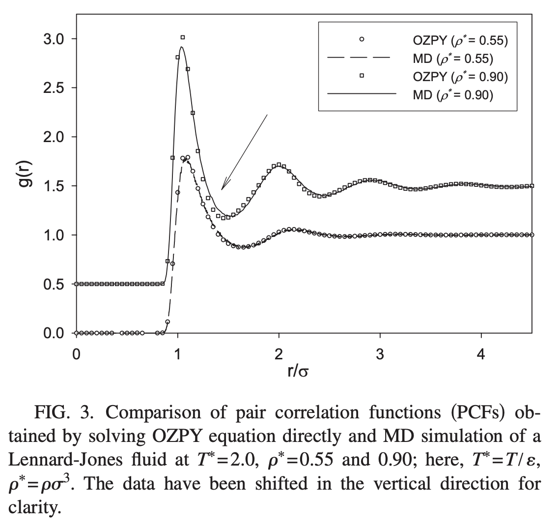
We can compare our results to the typical appearance of the correlation function for a dense packing of hard spheres. The correlation function is a smooth function that decays to one (the asymptotic average density) at long distances.
This figure from Wang et al. PRE 2010 shows the correlation function computed from molecular dynamics simulations, as well as an analytic approximate solution for g(r),
## Make an interactive video
from ipywidgets import interact
import ipywidgets as widgets


def plotter(i):
    coords = hsp.history[i]
    fig = plt.figure(figsize=(8,8))
    ax = fig.add_subplot(111, projection='3d')
    ax.scatter(coords[:, 0], coords[:, 1], coords[:, 2], c='b', marker='o', s=100, alpha=0.2)
    ax.set_zlim(-0.5, 0.5)
    plt.xlim([-0.5, 0.5])
    plt.ylim([-0.5, 0.5])

    plt.show()

interact(
    plotter,
    i=widgets.IntSlider(min=5, max=len(hsp.history)-1, step=1, value=0)
)
interactive(children=(IntSlider(value=5, description='i', max=1643, min=5), Output()), _dom_classes=('widget-i…
<function __main__.plotter(i)>
Questions
We have a double loop: an outer loop over all iterations, and an inner loop where we go over each individual particle, jostle it, and check for overlaps. Why can't this inner loop be vectorized?
How would we generalize this approach to a soft-repulsive potential?
from IPython.display import Image
Image("../resources/hardsphere_diagram.png", width=500)
# Computer simulations of dense hard‐sphere systems, Rintoul & Torquato. JCP 1996

What about long-range interactions?
For the hard-sphere system, we needed to compute the energy change based on the potentially-overlapping neighbors of each particle.
Locality: When a single particle position updates, we only need to check locally for potential new overlaps---we don't have to check particles that are across the lattice.
For N particles with volume $v$ in a volume $V$, the number density is $\rho = N/v$. The number of overlapping neighbors is therefore, on average, equal to $K = N v / V$.
The energy update for the hard-sphere potential therefore takes $O(N K)$ time to compute. Usually, $K \ll N$ and so we say the cost is $O(N)$. This is also true for soft-spheres, and it is effectively true for short-range potentials like the Lennard-Jones potential.
But what about gravitationally-interacting systems? For every update, we have to check interactions with every other particle. This is $O(N^2)$, and it is a major computational bottleneck for gravitational N-body simulations.
One solution involves using approximate force fields for long-range interactions. Examples of algorithms that do this include the Barnes-Hut algorithm, the Fast Multipole Method, and Ewald summation.
Further reading
A recent modification of the Metropolis algorithm by Muller et al., rearranges the acceptance step
$$ \Delta E = -\dfrac{\log \rho}{\beta} \equiv \Delta E_{th} $$
where $\rho$ is a random number between 0 and 1. This approach therefore re-frames the Metropolis update as determining whether the proposed energy change $\Delta E$ lies above or below the random threshold $\Delta E_{th}$.
The key insight of Müller et al. is that $\Delta E$ does not need to be known exactly. Rather, it is sufficient to gradually update a set of upper and lower bounds, $\Delta E \in [\Delta E_{min}, \Delta E_{max}]$. If $\Delta E_{min} < \Delta E_{th}$ then the update is accepted. If $\Delta E_{max} < \Delta E_{th}$ then the update is rejected probabilistically.
Thus, rather than exactly compute the energy change, the authors can use a tree-like decomposition of the domain to gradually improve bounds on the true energy change, until one of the stopping conditions above is triggered. Importantly, this is an exact algorithm, and it does not require any approximations.
From the Martiniani lab: basins of attraction video for soft repulsive particles