Evolving cellular automata with genetic algorithms

Preamble: Run the cells below to import the necessary Python packages

This notebook created by William Gilpin. Consult the course website for all content and GitHub repository for raw files and runnable online code.

import numpy as np

# Wipe all outputs from this notebook
from IPython.display import Image, clear_output, display
clear_output(True)

# Import local plotting functions and in-notebook display functions
import matplotlib.pyplot as plt
%matplotlib inline

# Add the course directory to the Python path
# import sys
# sys.path.append('../') 
# # import cphy.plotting as cplot

Gradient-free optimization

• We saw before that many optimization methods implicitly require the locally-computed gradient of the potential, either explicitly or a finite-difference approximation

• However, in many contexts this gradient is not available or is too expensive to compute

• Today, we will consider a case where the gradient is impossible to compute, because the underlying system is discrete

Genetic algorithms

• We define a set of candidate solutions to a problem, called the population

• We then iteratively select the best solutions from the population using a fitness function. The next generation will inherit properties these best solutions from the previous generation

• We use the best solutions to create new "offspring" solutions using a combination of mutation and crossover. The former corresponds to a random change in the solution, while the latter corresponds to combining two solutions to create a new one.

• The offspring solutions are then added to the population, and they usually replace the worst solutions

class GeneticAlgorithm:
    """
    Base class for genetic algorithms

    Parameters:
        population_size (int): Number of individuals in the population
        fitness_function (callable): Function that computes the fitness of an individual
        mutation_rate (float): Probability of mutating an individual
        crossover_rate (float): Probability of crossing over two individuals
        fraction_elites (float): Fraction of the population that is copied to the next generation
        random_state (int): Random seed
        verbose (bool): If True, print progress information during evolution
        store_history (bool): If True, store the fitness of the population at each 
            generation
    """

    def __init__(self, 
                 population_size, fitness_function, mutation_rate=0.1, 
                 crossover_rate=0.5, fraction_elites=0.5,
                 random_state=None, verbose=False, store_history=True
        ):
        self.population_size = population_size
        self.fitness_function = fitness_function
        self.mutation_rate = mutation_rate
        self.crossover_rate = crossover_rate
        self.fraction_elites = fraction_elites

        self.random_state = random_state
        np.random.seed(self.random_state)

        self.verbose = verbose
        self.store_history = store_history
        if self.store_history:
            self.history = list()

        ## Initialize internal variables
        self.population = None
        self.best_fitness = None
        self.best_individual = None


    def initialize(self):
        """Initialize a population of individuals"""
        raise NotImplementedError("This method must be implemented by a subclass")

    def step(self):
        """Perform a single update step of the entire population"""
        raise NotImplementedError("This method must be implemented by a subclass")

    def evolve(self, n_generations):
        """Evolve the population for a given number of generations"""
        self.initialize()
        for i in range(n_generations):
            if self.verbose:
                if i % (n_generations // 20) == 0:
                    print(f'Generation {i} of {n_generations}')
            self.step()
        return self.best_individual

To use genetic algorithms, we need to define a fitness function, which encodes the objective we want to optimize. Here, we will use a familiar low-dimensional fitness function that we saw in the context of gradient descent: the inverse Gaussian function.

def fitness(x):
    """A 2D fitness function corresponding to the sum of two Gaussian peaks"""
    return np.exp(-((x[0] - 0.5)**2 + (x[1] - 0.5)**2) / 0.1**2) + \
           np.exp(-((x[0] - 0.5)**2 + (x[1] - 0.75)**2) / 0.1**2)

xx, yy = np.meshgrid(np.linspace(0, 1, 100), np.linspace(0, 1, 100))
xx, yy = xx.ravel(), yy.ravel()

plt.figure(figsize=(6, 6))
plt.scatter(xx, yy, c=fitness([xx, yy]), s=10, cmap='viridis')
plt.axis('off')

(-0.05, 1.05, -0.05, 1.05)

class EvolveLandscape(GeneticAlgorithm):

    def __init__(self, *args, **kwargs):
        super().__init__(*args, **kwargs)

        self.population = np.random.rand(self.population_size, 2)

    def initialize(self):
        """Initialize a population of individuals"""
        self.best_fitness = np.zeros(self.population_size)
        self.best_individual = np.zeros(2)

    def step(self):
        """Perform a single update step of the entire population"""
        # Evaluate the fitness of each individual
        for i in range(self.population_size):
            self.best_fitness[i] = self.fitness_function(self.population[i])
        # Find the best individual
        self.best_individual = self.population[np.argmax(self.best_fitness)]
        # Store the best fitness
        if self.store_history:
            self.history.append(self.best_fitness.copy())

        # Create a new population
        new_population = np.zeros_like(self.population)

        # Copy the best individuals
        n_elites = int(self.fraction_elites * self.population_size)
        new_population[:n_elites] = self.population[np.argsort(self.best_fitness)][-n_elites:]
        # Fill the rest of the population by crossover
        for i in range(n_elites, self.population_size, 2):
            # Select two individuals from the current population
            parents = self.population[np.random.choice(self.population_size, 2, replace=False)]
            # Perform crossover
            new_population[i] = parents[0] * (1 - self.crossover_rate) + parents[1] * self.crossover_rate
            new_population[i + 1] = parents[1] * (1 - self.crossover_rate) + parents[0] * self.crossover_rate
            # Mutate the new individuals
            if np.random.rand() < self.mutation_rate:
                new_population[i] += np.random.randn(2) * 0.1
            if np.random.rand() < self.mutation_rate:
                new_population[i + 1] += np.random.randn(2) * 0.1
        # Replace the old population with the new one
        self.population = new_population

# Create an instance of the genetic algorithm
ga = EvolveLandscape(
    population_size=100, fitness_function=fitness, mutation_rate=0.1, 
    crossover_rate=0.5, fraction_elites=0.5, random_state=0, verbose=True
)

plt.figure(figsize=(6, 6))
plt.scatter(xx, yy, c=fitness([xx, yy]), s=10, cmap='viridis')
plt.scatter(ga.population[:, 0], ga.population[:, 1], c='r', s=10)
plt.title("Initial Population Positions")
plt.axis('off')

# Evolve the population for 100 generations
ga.evolve(100)

plt.figure(figsize=(6, 6))
plt.scatter(xx, yy, c=fitness([xx, yy]), s=10, cmap='viridis')
plt.scatter(ga.best_individual[0], ga.best_individual[1], c='r', s=100, marker='*')
plt.scatter(ga.population[:, 0], ga.population[:, 1], c='r', s=10)
plt.title("Final Population Positions")
plt.axis('off')

# Plot the fitness of the population over time
plt.figure()
plt.plot(np.min(ga.history, axis=1), label="Min Fitness")
plt.plot(np.mean(ga.history, axis=1), label="Mean Fitness")
plt.plot(np.max(ga.history, axis=1), label="Max Fitness")
plt.legend()
plt.xlabel("Generation")
plt.ylabel("Fitness")

Generation 0 of 100
Generation 5 of 100
Generation 10 of 100
Generation 15 of 100
Generation 20 of 100
Generation 25 of 100
Generation 30 of 100
Generation 35 of 100
Generation 40 of 100
Generation 45 of 100
Generation 50 of 100
Generation 55 of 100
Generation 60 of 100
Generation 65 of 100
Generation 70 of 100
Generation 75 of 100
Generation 80 of 100
Generation 85 of 100
Generation 90 of 100
Generation 95 of 100

Text(0, 0.5, 'Fitness')

Evolving cellular automata

• Cellular automata take discrete values, and update on a discrete grid in discrete time steps

• This discrete nature precludes the use of gradient-based methods when analyzing their behavior

Influential results that exploring the space of CA with genetic algorithms can be found in Mitchell et al. 1993 and Crutchfield & Mitchell 1995

We start by defining our base class for cellular automata, which should look familiar from the previous notebook.

class CellularAutomaton:
    """
    A base class for cellular automata. Subclasses must implement the step method.

    Parameters
        n (int): The number of cells in the system
        n_states (int): The number of states in the system
        random_state (None or int): The seed for the random number generator. If None,
            the random number generator is not seeded.
        initial_state (None or array): The initial state of the system. If None, a 
            random initial state is used.
        
    """
    def __init__(self, n, n_states, random_state=None, initial_state=None):
        self.n_states = n_states
        self.n = n
        self.random_state = random_state

        np.random.seed(random_state)

        ## The universe is a 2D array of integers
        if initial_state is None:
            self.initial_state = np.random.choice(self.n_states, size=(self.n, self.n))
        else:
            self.initial_state = initial_state
        self.state = self.initial_state

        self.history = [self.state]

    def next_state(self):
        """
        Output the next state of the entire board
        """
        return NotImplementedError

    def simulate(self, n_steps):
        """
        Iterate the dynamics for n_steps, and return the results as an array
        """
        for i in range(n_steps):
            self.state = self.next_state()
            self.history.append(self.state.copy())
        return self.state

We want to represent the space of rules, which are discrete-valued functions that take in a neighborhood of cells and return a new value for the center cell

• We consider only binary cellular automata like Conway's Game of Life, for which a given cell can be either "alive" (1) or "dead" (0)

• For a Moore neighborhood CA (nearest neighbors including diagonal), there are $2^9 = 512$ possible input values if we include the center cell

• For each input value, there are two possible output values. Therefore, there are $2^{2^9} \approx 10^{154}$ possible rules.

We therefore define a subclass, ProgrammaticCA, which takes a ruleset in its constructor and defines the corresponding CA. We saw previously that many common CA may be quickly implemented using 2D convolutions with an appropriate kernel. For our implementation, we define a special convolutional kernel that converts a 3x3 neighborhood into a unique integer between 0 and 511. We then use this integer to index into the ruleset to determine the output value.

from scipy.signal import convolve2d

class ProgrammaticCA(CellularAutomaton):

    def __init__(self, n, ruleset,  **kwargs):
        k = np.unique(ruleset).size
        super().__init__(n, k, **kwargs)
        self.ruleset = ruleset

        ## A special convolutional kernel for converting a binary neighborhood 
        ## to an integer
        self.powers = np.reshape(2 ** np.arange(9), (3, 3))

    def next_state(self):

        # Compute the next state
        next_state = np.zeros_like(self.state)
        
        # convolve with periodic boundary conditions
        rule_indices = convolve2d(self.state, self.powers, mode='same', boundary='wrap')

        ## look up the rule for each cell
        next_state = self.ruleset[rule_indices.astype(int)]

        return next_state

# An entire CA can be represented as a single binary integer or hexidecimal code
random_ruleset = np.random.choice(2, size=2**9)

model = ProgrammaticCA(100, random_ruleset, random_state=0)
model.simulate(500)

plt.figure()
plt.imshow(model.initial_state, cmap="gray")
plt.title("Initial state")

plt.figure()
plt.imshow(model.state, cmap="gray")
plt.title("Final state")

Text(0.5, 1.0, 'Final state')

Searching the space of cellular automata with genetic algorithms

We are now ready to define a genetic algorithm that searches the space of cellular automata for interesting behavior.

Our fitness function will encode the desired properties of a learned automaton.

• A simple choice is the variance of the number of live vs dead cells, in order to encourage discovery of CA that produce long-lived structures.

• We've made some modifications to encourage activity, but you can try changing the fitness function to see what happens.

def fitness(trajectory):
    """
    A fitness function that rewards activity (mixtures of on and off cells)

    Args:
        trajectory (array): A 2D array of integers representing the state of the CA at
            each time step of the simulation. Shape is (n_steps, nx, ny)

    Returns:
        float: A fitness score
    """
    final_state = trajectory[-1]            
    timechange = np.sum(np.abs(np.diff(np.array(trajectory), axis=0)))
    timechange /= final_state.size
    return np.max(final_state) - np.min(final_state) - np.std(final_state) + timechange

Our genetic algorithm will contain the following steps:

1. The initialize method initializes a population of individuals, which are represented by binary strings describing their rulesets

2. The step method loops over each individual in the population and creates a CA with its ruleset. It then runs the CA for a fixed number of time steps and computes the fitness from the trajectory. The fitness is then stored in the fitnesses array. Selection is then performed using elitism, crossover, and mutation.

All other methods are deferred to the base class.

class EvolveCA(GeneticAlgorithm):
    """
    A class for evolving cellular automata rulesets using a genetic algorithm

    Parameters
        n_size (int): The size of the CA spatial lattice
        n_steps (int): The number of CA steps to simulate per generation (the 
            trajectory length)
        **kwargs: Keyword arguments to pass to the GeneticAlgorithm superclass
    """

    def __init__(self, n_size, n_steps, **kwargs):
        super().__init__(**kwargs)
        self.n_size = n_size
        self.n_steps = n_steps

    def initialize(self):
        self.population = np.random.choice(2, size=(self.population_size, 2**9))

    def step(self):
        """Evolve one generation of the population"""
        fitnesses = []
        for ruleset in self.population:
            model = ProgrammaticCA(self.n_size, ruleset, random_state=0)
            model.simulate(self.n_steps)

            fitness_val = self.fitness_function(model.history)
            fitnesses.append(fitness_val)
        fitnesses = np.array(fitnesses)

        if self.store_history:
            self.history.append(fitnesses)

        ## Sort population by fitness
        self.population = self.population[np.argsort(fitnesses)]

        ## Create a new generation
        n_elite = int(self.fraction_elites * self.population_size)
        for i in range(self.population_size - n_elite):
            
            ## Crossover two high-performing rulesets
            parent1_ind, parent2_ind = np.random.choice(
                len(self.population[-n_elite:]), size=2, replace=True
            )
            parent1 = self.population[-n_elite:][-parent1_ind]
            parent2 = self.population[-n_elite:][-parent2_ind]
            crossover_point = np.random.randint(len(parent1))

            # crossover_point = 0
            child = np.hstack((parent1[:crossover_point], parent2[crossover_point:]))

            ## Mutate the child at random points
            n_mutate = int(self.mutation_rate * len(child))
            child[np.random.randint(2**9, size=n_mutate)] = np.random.randint(2, size=n_mutate)

            self.population[i] = child
        self.best_individual = self.population[-1]
        self.best_fitness = np.max(fitnesses)

evolver = EvolveCA(40, 40, population_size=1000, fitness_function=fitness, random_state=0, verbose=True)
evolver.evolve(1000)

plt.figure()
plt.plot(np.min(evolver.history, axis=1), label="Min Fitness")
plt.plot(np.mean(evolver.history, axis=1), label="Mean Fitness")
plt.plot(np.max(evolver.history, axis=1), label="Max Fitness")
plt.legend()
plt.xlabel("Generation")
plt.ylabel("Fitness")

Generation 0 of 1000
Generation 50 of 1000
Generation 100 of 1000
Generation 150 of 1000
Generation 200 of 1000
Generation 250 of 1000
Generation 300 of 1000
Generation 350 of 1000
Generation 400 of 1000
Generation 450 of 1000
Generation 500 of 1000
Generation 550 of 1000
Generation 600 of 1000
Generation 650 of 1000
Generation 700 of 1000
Generation 750 of 1000
Generation 800 of 1000
Generation 850 of 1000
Generation 900 of 1000
Generation 950 of 1000

Text(0, 0.5, 'Fitness')

digit_5 = np.array([
    [0, 0, 0, 0, 0, 0, 0, 0, 0, 0],
    [0, 0, 0, 0, 0, 0, 0, 0, 0, 0],
    [0, 0, 0, 1, 1, 1, 1, 0, 0, 0],
    [0, 0, 0, 1, 0, 0, 0, 0, 0, 0],
    [0, 0, 0, 1, 1, 1, 0, 0, 0, 0],
    [0, 0, 0, 0, 0, 0, 1, 0, 0, 0],
    [0, 0, 0, 0, 0, 0, 1, 0, 0, 0],
    [0, 0, 0, 1, 1, 1, 0, 0, 0, 0],
    [0, 0, 0, 0, 0, 0, 0, 0, 0, 0],
    [0, 0, 0, 0, 0, 0, 0, 0, 0, 0]
])
# digit_5 = np.logical_not(digit_5)


model = ProgrammaticCA(10, evolver.best_individual, random_state=0, initial_state=digit_5)
model.simulate(30)

plt.figure()
plt.imshow(model.initial_state, cmap="gray")
plt.axis("off")
plt.title("Initial state")


plt.figure()
plt.imshow(model.state, cmap="gray")
plt.axis("off")
plt.title("Final state")

Text(0.5, 1.0, 'Final state')

from matplotlib.animation import FuncAnimation
from IPython.display import HTML

# Assuming frames is a numpy array with shape (num_frames, height, width)
frames = np.array(model.history).copy() 

fig = plt.figure(figsize=(6, 6))
img = plt.imshow(frames[0], vmin=0, vmax=1, cmap="gray");
plt.xticks([]); plt.yticks([])
# tight margins
plt.margins(0,0)
plt.gca().xaxis.set_major_locator(plt.NullLocator())

def update(frame):
    img.set_array(frame)

ani = FuncAnimation(fig, update, frames=frames, interval=200)
HTML(ani.to_jshtml())

Once Loop Reflect

Outlook

Genetic algorithms can be found in many contexts where the "inverse" problem is difficult to solve. For example, they can be used to design meterials with desired properties, to optimize the design of mechanical structures like bridges, or even to perform hyperparameter optimization for machine learning models.

For example a recent study uses GA to design a metamaterial that exhibits nearly optimal optical absorption over a given wavelength range.

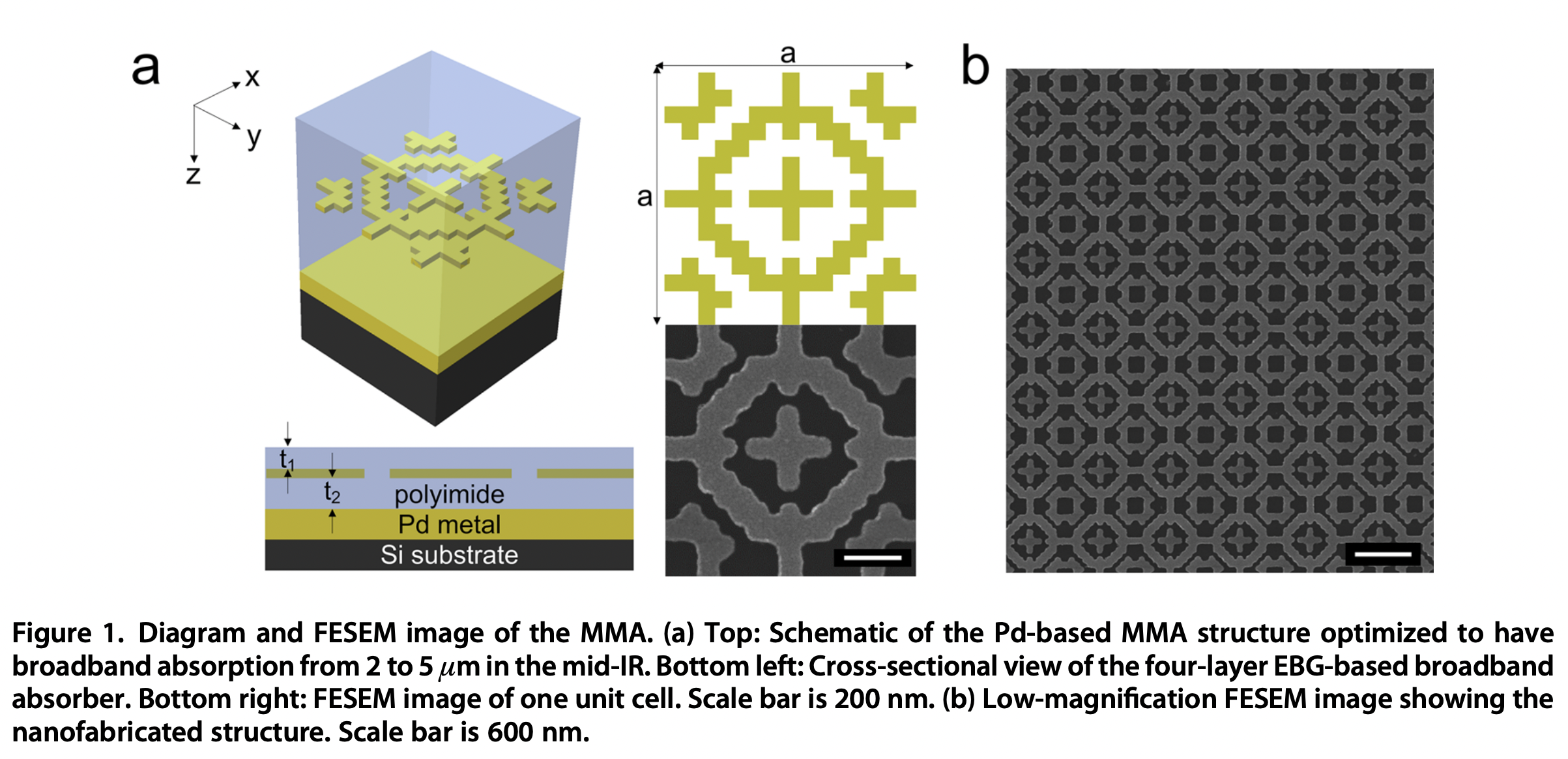
Image from Bossard et al. 2014

Appendix: Hyperparameters to modify

• Single-rule crossovers

• Fewer mutations