Optimization in many dimensions - An Introduction to Algorithms for Physicists

Previously, we considered optimization of functions that depend on a single variable. In this notebook, we will consider optimization of functions that depend on many variables, which describes many physical systems as well as many machine learning problems. Several approaches from univariate optimization, like gradient descent, can be extended to the multivariate case, but new methods are also needed because the landscape of a multivariate function is much more complex than that of a univariate function. We will conclude by implementing minimal versions of modern optimizers, like L-BFGS and Adam, which are widely used in machine learning.

Preamble: Run the cells below to import the necessary Python packages

import numpy as np
from IPython.display import Image, display

import matplotlib.pyplot as plt
%matplotlib inline

## Set nicer colors
plt.rcParams['image.cmap'] = 'PuBu'
plt.rcParams['axes.prop_cycle'] = plt.cycler(color=[[1.0, .3882, .2784]])
plt.rcParams['lines.markersize'] = 10

## Comment out these lines if they throw an error on your system
## Set animation parameters
## Tune the ffmpeg writer (you need ffmpeg installed)
plt.rcParams["animation.writer"] = "ffmpeg"
plt.rcParams["animation.bitrate"] = 800                     # kb/s cap
plt.rcParams["animation.ffmpeg_args"] = [                   # finer control
    "-crf", "24",        # 18–28 is common; larger = smaller file
    "-preset", "slow",   # slower = better compression
    "-pix_fmt", "yuv420p"
]
plt.rcParams["animation.embed_limit"] = 25

A Gaussian landscape¶

We will optimize a two-dimensional landscape consisting of a sum of Gaussian wells,

\mathcal{L}_{\boldsymbol{\mu}, \boldsymbol{\sigma}}(\mathbf{x}) = \sum_{p=1}^P \mathcal{L}_p = -\sum_{p=1}^P A_p \exp\left(-\frac{(\mathbf{x} - \boldsymbol{\mu}_{p})^2}{2\sigma^2}\right)

(1)

where $\mathbf{x} \in \mathbb{R}^D$ is the position in the landscape, $\boldsymbol{\mu}_p \in \mathbb{R}^D$ is the location of the $p^{th}$ well, and $\sigma \in \mathbb{R}^D$ is the width of the wells. The weights $\sum_p A_p = 1$ , $A_p \geq 0$ are the relative depths of the wells.

Implementing the random landscape. Recall that, during optimization, we usually think of our “cost” as being the number of calls to the function we are trying to optimize. Here, to implement this landscape, we will make calculating its value at a single point as fast as possible using vectorization. Since the well positions are all fixed, and the landscape is a sum over them, we can vectorize this sum rather than writing an explicit loop over the index $p$ . Additionally, if we want to calculate the landscape value at $N$ different points in space at once, we broadcast across different $\mathbf{x}$ values, because the different evaluations are independent of each other.


class RandomLossLandscapeWithoutGradient:
    """
    Creates a random two-dimensional loss landscape with multiple circular gaussian wells

    Args:
        d (int): number of dimensions for the loss landscape
        n_wells (int): number of gaussian wells
        random_state (int): random seed
    
    """

    def __init__(self, d=2, n_wells=3, random_state=None):
        
        # Fix the random seed
        self.random_state = random_state
        np.random.seed(random_state)

        # Select random well locations, widths, and amplitudes
        self.locs = (2 * np.random.uniform(size=(n_wells, d)) - 1) * 3
        self.widths = np.random.rand(n_wells)[None, :]
        self.coeffs = np.random.random(n_wells)
        self.coeffs /= np.sum(self.coeffs) # normalize the amplitudes

    def _gaussian_well(self, X, width=1):
        """
        A single gaussian well centered at 0 with specified width

        Args:
            X (np.ndarray): points at which to compute the gaussian well. This should 
                be of shape (n_batch, n_dim)
            width (float): The width of the gaussian well

        Returns:
            np.ndarray: The value of the gaussian well at points X. The shape of the output
                is (n_batch,)
        """
        return -np.exp(-np.sum((X / width) ** 2, axis=1))
    
    def loss(self, X):
        """
        Compute the loss landscape at points X

        Args:
            X (np.ndarray): points at which to compute the loss landscape. This should 
                be of shape (n_batch, n_dim)
            width (float): The width of the gaussian wells

        Returns:
            np.ndarray: loss landscape at points X

        Notes:
            The loss landscape is computed as the sum of the individual gaussian wells
            The shape of the argument to np.sum is (n_batch, n_wells)
        """
        # print(X[..., None].shape)
        # print(self.locs.shape)
        # print(self.locs.T[None, :].shape)
        # print((X[..., None] - self.locs.T[None, :]).shape)
        # print((self._gaussian_well(X[..., None] - self.locs.T[None, :])).shape)
        return np.sum(
            self._gaussian_well(X[..., None] - self.locs.T[None, :], self.widths) * self.coeffs,
            axis=1
        )

    def __call__(self, X):
        return self.loss(X)


loss = RandomLossLandscapeWithoutGradient(random_state=0, n_wells=8)

## specify three positions in a 2D space
X = np.array([[0, 0], [1, 1], [-1, -1], [-1, -.5]])
print(X.shape)
loss(X)

(4, 2)

array([-0.09565806, -0.0812864 , -0.00054421, -0.00266954])

Our implementation is vectorized, and so we can pass multiple points at once and compute the loss for all of them very quickly.

loss(np.array([[0.1, 0.3], [0.1, 0.7]]))

array([-0.12900234, -0.11453241])

We can now plot the landscape by evaluating the loss $\mathcal{L}$ at a grid of points. Because our function is vectorized, we pass a single array $X \in \mathbb{R}^{N \times D}$ and get back a vector of length $N$ containing the scalar loss at each point. We then plot this scalar field as a color plot versus the original positions $X$ .

## We have to make a list of points at which to plot the landscape. NumPy's meshgrid is 
## a built-in utility for this purpose. 
x = np.linspace(-3, 3, 100)
y = np.linspace(-3, 3, 100)
xx, yy = np.meshgrid(x, y)
X = np.array([xx.ravel(), yy.ravel()]).T
print(X.shape)
Z = loss(X) # same as loss.loss(X) because class is callable

plt.figure(figsize=(8, 8))
plt.scatter(X[:, 0], X[:, 1], c=Z)
plt.plot(xx.ravel()[Z.argmin()], yy.ravel()[Z.argmin()], '*', markersize=20)
plt.axis('off')

(10000, 2)

(np.float64(-3.3), np.float64(3.3), np.float64(-3.3), np.float64(3.3))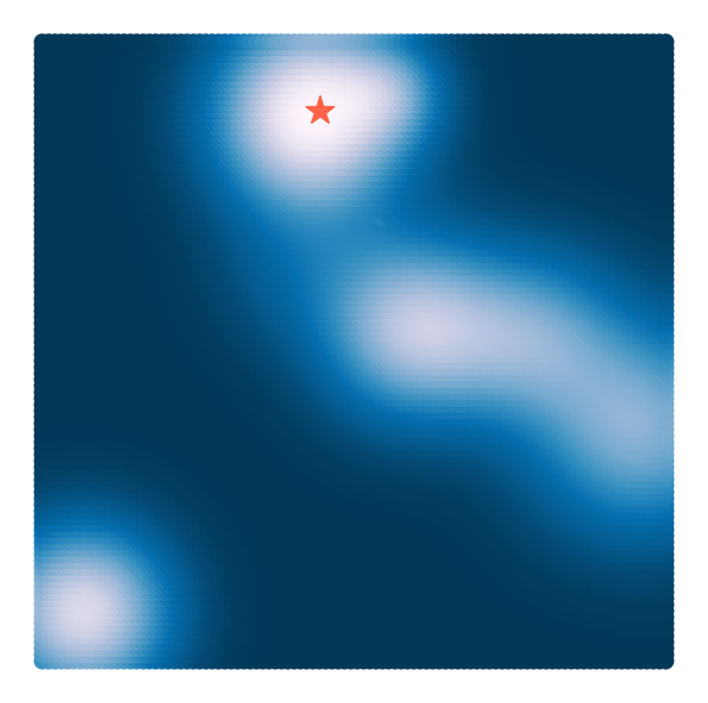

Recall that many optimization routines requre the gradient of the landscape. We can analytically calculate the gradient of this landscape

\mathcal{L} = \sum_{p=1}^P \mathcal{L}_p = -\sum_{p=1}^P A_p \exp\left(-\frac{(\mathbf{x} - \boldsymbol{\mu}_{p})^2}{2\sigma^2}\right)

(2)

\nabla \mathcal{L} = \sum_{p=1}^P A_p\frac{(\mathbf{x} - \boldsymbol{\mu}_{p})}{\sigma^2} \exp\left(-\frac{(\mathbf{x} - \boldsymbol{\mu}_{p})^2}{2\sigma^2}\right)

(3)

Recall that while $\mathcal{L}$ is a scalar, $\nabla \mathcal{L}$ is a vector of the same dimension as $\mathbf{x}$ . We can implement both the landscape and its gradient within a single loss object. We vectorize the computation of the loss and gradient over the $P$ wells using np.einsum

class RandomLossLandscape(RandomLossLandscapeWithoutGradient):
    """
    A random two-dimensional loss landscape with a gradient defined everywhere
    """

    def __init__(self, *args, **kwargs):
        ## Passes all arguments and keyword arguments to the parent class
        super().__init__(*args, **kwargs)

    def _grad_gaussian_well(self, X, width=1):
        return -2 * X / (width ** 2) * self._gaussian_well(X, width)[:, None, :]

    def grad(self, X):
        # Arg shape before summation is (n_batch, n_dim, n_wells)
        return np.sum(
            self.coeffs * self._grad_gaussian_well(X[..., None] - self.locs.T[None, :], self.widths), 
            axis=-1
        )

loss = RandomLossLandscape(random_state=0, n_wells=8)

plt.figure(figsize=(8, 8))

## First we plot the scalar field at high resolution
x = np.linspace(-3, 3, 100)
y = np.linspace(-3, 3, 100)
xx, yy = np.meshgrid(x, y)
X = np.array([xx.ravel(), yy.ravel()]).T
print(X.shape)
Z = loss(X) # same as loss.loss(X) because class is callable
plt.scatter(X[:, 0], X[:, 1], c=Z, s=1000)

# x = np.linspace(-3, 3, 15)
# y = np.linspace(-3, 3, 15)
# xx, yy = np.meshgrid(x, y)
# X = np.array([xx.ravel(), yy.ravel()]).T
# Z = loss.loss(X)
plt.quiver(X[:, 0], X[:, 1], loss.grad(X)[:, 0], loss.grad(X)[:, 1], scale=1e1, color='k')
plt.axis('off')

(10000, 2)

(np.float64(-3.3), np.float64(3.3), np.float64(-3.3), np.float64(3.3))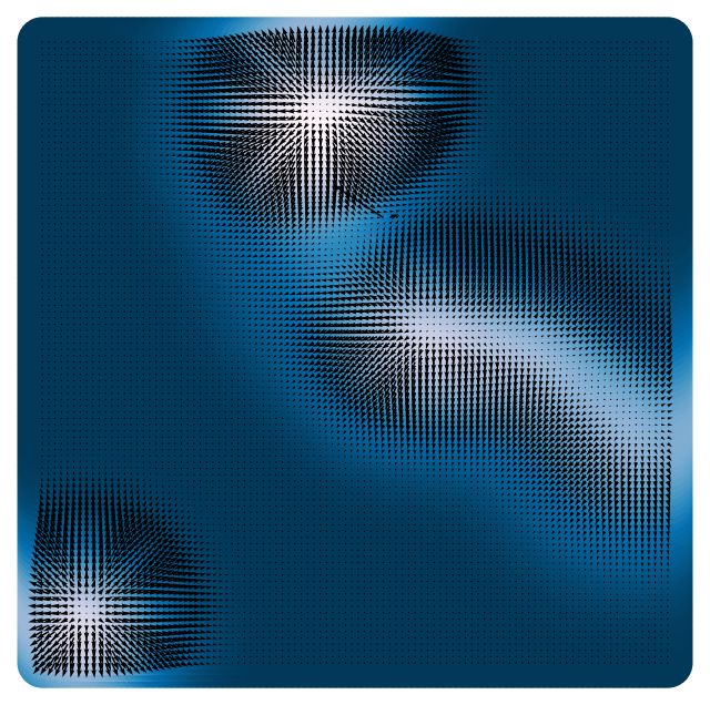

Disordered media and Gaussian Random Fields¶

The Gaussian mixture we are studying is a toy model for disordered media, because it approximates Gaussian random field (GRF). A GRF is a random function $f(x)$ whose values at any set of points $x_1, x_2, \ldots, x_n$ are jointly Gaussian distributed. This means that the probability distribution for the values of the function at these points is given by a multivariate normal distribution.

Gaussian random fields appear as models in many areas of physics and engineering, including:

Cosmology: The initial density fluctuations in the early universe are often modeled as a Gaussian random field.
Geostatistics: GRFs are used to model spatially correlated data, such as the distribution of minerals in the Earth’s crust or the variation of soil properties.
Condensed Matter Physics: GRFs can describe disordered systems, such as spin glasses or random media.

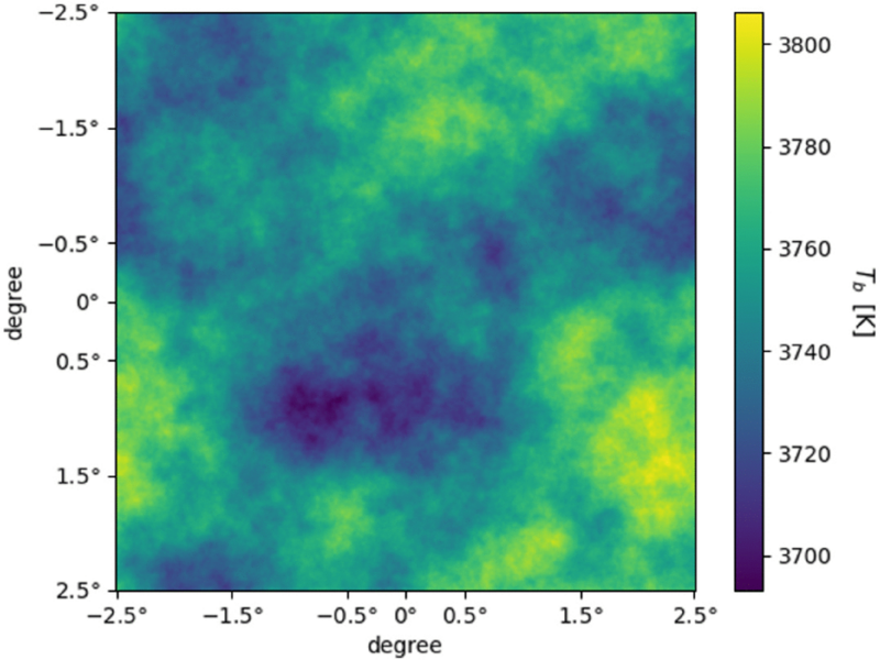
Gaussian random fields are used to model brightness fluctuations in radio spectrum in models of the early universe. Image from Maibach et al., Phys. Rev. D (2021).

Optimization in complex landscapes¶

We are interested in finding the minima of a Gaussian random field. In a disordered system like a material, this corresponds to where the system localizes at low temperatures.

Some considerations when performing multivariate optimization¶

Having a smooth landscape is important for many optimization algorithms to work well, because gradient information is required for local search methods to update their state in a meaningful way.
Because differentiability is a concern, we expect that flatter regions in the landscape will pose challenges. In our Gaussian landscape, the regions far away from the $P$ centers will be flat, and so we expect optimizers initialized in these regions to struggle on this problem.

Computing analytic gradients is hard¶

Computing analytic gradients is hard, and often impossible. We can use finite differences to approximate the gradient along each dimension:

\frac{\partial f}{\partial x_i} \approx \frac{f(x_1, \ldots, x_i + \epsilon, \ldots, x_D) - f(x_1, \ldots, x_i - \epsilon, \ldots, x_D)}{2\epsilon}

(4)

Finite difference gradients are computationally expensive: In $d$ dimensions, we need to evaluate the function $\mathcal{O}(d)$ times to compute the gradient. This is impractical for high-dimensional problems, but it is acceptable for our 2D landscape.
Symbolic gradients are useful, but prone to errors
We use a gradcheck function to mitigate the risk of errors in our gradients.
(Later in the course): Faster gradient estimation for more complex loss functions with automatic differentiation (the symbolic chain rule for arbitrary compositions of primitive functions).

def gradcheck(loss, x, eps=1e-9):
    """
    This function computes the exact gradient and an approximate gradient using 
    finite differences

    Args:
        loss (callable): loss function. Must have a method `grad` that returns the 
            analytic gradient
        x (np.ndarray): input to the loss function
        eps (float): epsilon for finite differences

    Returns:
        grad (np.ndarray): analytic gradient
        grad_num (np.ndarray): numerical gradient
    
    """
    x = np.array(x)
    grad = loss.grad(x)
    grad_num = list()
    for i in range(x.shape[0]):
        x1, x2 = x.copy(), x.copy()
        x1[i] += eps
        x2[i] -= eps
        grad_num.append((loss(x1) - loss(x2)) / (2 * eps))
    grad_num = np.array(grad_num)
    return grad, grad_num

grad, grad_num = gradcheck(loss, np.random.randn(2))

print(f"True gradient: {grad.squeeze()}\nApproximate gradient: {grad_num.squeeze()}")

print(np.allclose(grad, grad_num, atol=1e-1))

True gradient: [ 0.07939433 -0.0170474 ]
Approximate gradient: [ 0.07939433 -0.0170474 ]
True

Why not use global methods?¶

Why bother using gradient descent when we can just check every point in our system’s domain? That’s literally how we generated the plot above.
For a continuous field, we need to pick some minimum length scale over which we don’t expect the objective to change rapidly. For discrete optimization, we just try all combinations
Assume we need $N$ points to sample along any linear dimension. The number of queries to the objective function scales as $N^d$ , where $d$ is the dimensionality
- For the example we just used, we sampled $N = 100$ points along each dimension, resulting in $100^2 = 10^4$ function calls.
- Assuming 100 points per axis, when $d = 3$ we have 10⁶ while for $d = 7$ it takes 10¹⁴, etc
- Let’s assume it takes 10 $\mu s$ per evaluation. The 2D global search takes 0.1 s, the 3D search takes 10 s, the $d = 5$ search takes 1.15 days, and the $d = 7$ search takes 32 years
What is a typical value of $d$ ? OpenAI’s DallE image generation model contains 12 billion parameters ( $d \approx 10^{10}$ ).

x = np.linspace(-3, 3, 100)
y = np.linspace(-3, 3, 100)
xx, yy = np.meshgrid(x, y)
X = np.array([xx.ravel(), yy.ravel()]).T
Z = loss(X) # same as loss.loss(X) because class is callable

plt.figure(figsize=(8, 8))
plt.scatter(X[:, 0], X[:, 1], c=Z, s=2000)
plt.plot(xx.ravel()[Z.argmin()], yy.ravel()[Z.argmin()], '*r', markersize=10)
plt.axis('off')

(np.float64(-3.3), np.float64(3.3), np.float64(-3.3), np.float64(3.3))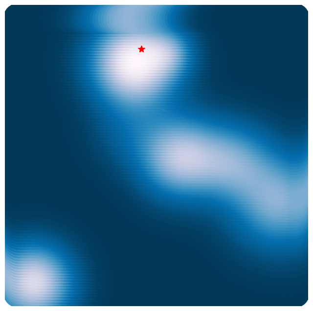

Optimizing in many dimensions¶

We will now implement a series of optimization algorithms to find the minima of our Gaussian mixture landscape
We will first define a base class for our optimizers, which will contain the common functionality of all optimizers. Many optimization algorithms are iterative, meaning that they start out at some (usually randomly-chosen) point on the landscape, and then incrementally update their position in order to reach the minimum.
The constructor will take a loss function itself, a learning rate that controls the rate of iterative updating, a maximum number of iterations, a tolerance that determines how close the optimization needs to get to a minimum to stop, a random seed, and a flag to store the history of steps taken during optimization
The base class will contain a fit method that will perform the optimization, and a update method that will be implemented by each subclass

class BaseOptimizer:
    """A Base class for multivariate optimizers
    
    Args:
        loss (callable): loss function. Must have a method `grad` that returns the 
            analytic gradient
        lr (float): learning rate
        max_iter (int): maximum number of iterations
        tol (float): tolerance for stopping criterion
        random_state (int): random seed
        store_history (bool): whether to store the optimization trajectory
    """

    def __init__(self, loss, lr=0.1, max_iter=1000, tol=1e-6, random_state=None, store_history=False):
        self.loss = loss
        self.lr = lr
        self.max_iter = max_iter
        self.tol = tol
        self.random_state = random_state
        np.random.seed(random_state)
        self.store_history = store_history
        if self.store_history:
            self.Xs = []
            self.losses = []

    def fit(self, X):
        """Minimize the loss function starting from a batch of initial guesses

        Args:
            X (np.ndarray): initial guess for the optimizer. Shape (n_dim,) or
                (n_batch, n_dim) if we have multiple initial points

        Returns:
            self
        """
        
        self.X = X
        if self.store_history:
            self.Xs = [self.X.copy()]
            self.losses = [self.loss(X)]
        for i in range(self.max_iter):
            
            self.X = self.update(self.X)

            if self.store_history:
                self.Xs.append(self.X.copy())
                self.losses.append(self.loss(self.X))

            # Stop early if loss is not decreasing any more for *any* batch elements
            if np.linalg.norm(self.loss.grad(self.X)) < self.tol:
                break

        return self
    
    def update(self, X):
        raise NotImplementedError("Implement this method in a subclass")

Multivariate gradient descent¶

A first-order optimization method because it only requires the first partial derivatives of the objective function
If we assume that our current position is $\mathbf{x}$ , then the gradient of the objective function at this point is $\nabla \mathcal{L}(\mathbf{x})$
The gradient descent update rule becomes
$\mathbf{x} \leftarrow \mathbf{x} - \eta \nabla \mathcal{L}(\mathbf{x})$
(5)
where $\eta$ is a step size parameter we call the “learning rate” that determines the size of the step we take in the direction of the gradient


class GradientDescent(BaseOptimizer):
    """A Multivariate Gradient Descent Optimizer"""

    def update(self, X):
        return X - self.lr * self.loss.grad(X)

We can now use this optimizer to find the minima of our two-dimensional Gaussian mixture landscape.

# Initialize optimizer
optimizer = GradientDescent(loss, lr=1e-1, max_iter=2000, tol=1e-6, random_state=0, store_history=True)

# Initialize many starting points
X0 = 6 * np.random.random(size=(100, 2)) - 3

# Fit optimizer
optimizer.fit(X0.copy())

<__main__.GradientDescent at 0x13671e350>

x = np.linspace(-3, 3, 100)
y = np.linspace(-3, 3, 100)
xx, yy = np.meshgrid(x, y)
X = np.array([xx.ravel(), yy.ravel()]).T
Z = loss.loss(X)

plt.figure(figsize=(8, 4))
plt.subplot(1, 2, 1)
plt.scatter(X[:, 0], X[:, 1], c=Z)
plt.plot(*X0.T, '.')
plt.xlim([-3, 3])
plt.ylim([-3, 3])
plt.axis('off')
plt.title('Initial Guesses')

plt.subplot(1, 2, 2)
Xs = np.array(optimizer.Xs)
plt.scatter(X[:, 0], X[:, 1], c=Z)
plt.plot(Xs[0, :, 0], Xs[0, :, 1], '.');
plt.plot(Xs[:, :, 0], Xs[:, :, 1], '-');
plt.plot(Xs[-1, :, 0], Xs[-1, :, 1], '.b', zorder=10);
plt.xlim([-3, 3])
plt.ylim([-3, 3])
plt.axis('off')
plt.title('Trajectories')

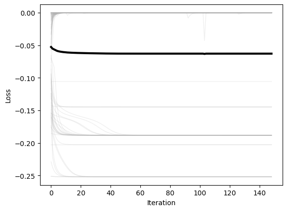
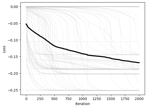
We next plot the loss versus time for each of the starting positions. We can also average the losses over the starting positions, in order to see how the loss evolves over time for a “typical” starting position.

plt.figure()
plt.plot(optimizer.losses, color=(0.7, 0.7, 0.7), lw=1, alpha=0.2)
plt.plot(np.mean(optimizer.losses, axis=1), 'k', lw=3)
plt.xlabel('Iteration')
plt.ylabel('Loss')

from matplotlib.animation import FuncAnimation
from matplotlib.collections import LineCollection
from IPython.display import HTML

Xs = np.array(optimizer.Xs)[::2][:500]

fig, ax = plt.subplots(figsize=(6, 6))
# ax.scatter(X[:, 0], X[:, 1], c=Z, s=14, zorder=0)
plt.imshow(Z.reshape(100, 100), extent=[-3, 3, -3, 3], origin='lower')
ax.plot(Xs[0, :, 0], Xs[0, :, 1], '.', ms=6, linestyle='None', zorder=1)
curr = ax.scatter([], [], s=20, c='b', zorder=3)
trail = LineCollection([], zorder=2)
ax.add_collection(trail)

ax.set_xlim(-3, 3); ax.set_ylim(-3, 3); ax.axis('off')
plt.margins(0, 0); plt.gca().xaxis.set_major_locator(plt.NullLocator())
plt.gca().yaxis.set_major_locator(plt.NullLocator())

def init():
    curr.set_offsets(np.array([0, 0]))
    trail.set_segments([])
    return (curr, trail)

def update(t):
    # current points
    curr.set_offsets(Xs[t])

    if t > 0:
        segs = []
        # Build one polyline per particle (skip if fewer than 2 points)
        for n in range(Xs.shape[1]):
            path = Xs[:t+1, n, :]  # (k,2)
            if path.shape[0] >= 2:
                segs.append(path)
        trail.set_segments(segs)


    return (curr, trail)

ani = FuncAnimation(fig, update, frames=min(500, Xs.shape[0]),
                    init_func=init, interval=100, blit=True, repeat=True)
html = ani.to_html5_video()                                 # replaces to_jshtml()
HTML(html)

Hyperparameter tuning: What is the correct learning rate?¶

Hyperparameter tuning is a big deal in machine learning.
For now, we will use intuition and trial-and-error to see how the learning rate and other hyperparameters affect the dynamics of the system
Many optimizers have multiple hyperparameters, and it is important to understand how these affect the dynamics of the system.

Momentum and stochasticity¶

We can think of gradent descent as the dynamics of a first-order overdamped system acting on a particle of mass $m$ in a potential $V(\mathbf{x})$ . For a particle of mass $m$ in a potential $V(\mathbf{x})$ , the forces acting on the particle are given by Newton’s second law:

\mathbf{F} = -\nabla \mathcal{U}(\mathbf{x})

(6)

\mathbf{a} = \frac{\mathbf{F}}{m}

(7)

If we assume linear damping with a damping coefficient $\gamma$ , then the dynamics of the particle are given by the kinematic equation:

m \ddot{\mathbf{x}} = -\gamma \dot{\mathbf{x}} - \nabla \mathcal{U}(\mathbf{x})

(8)

where $\mathbf{F}$ is the force, $\mathbf{a}$ is the acceleration. If we assume $\gamma \gg m$ , then the overdamped dynamics are given by the first-order equation of motion:

\dot{\mathbf{x}} = -\frac{1}{\gamma}\nabla \mathcal{U}(\mathbf{x})

(9)

In discrete time, the derivatives $\dot{\mathbf{x}}$ can be approximated using finite differences:

\dot{\mathbf{x}} \approx \frac{\mathbf{x}_{t+1} - \mathbf{x}_t}{\Delta t}

(10)

In discrete time, this equation corresponds to the update rule:

\mathbf{x}_{t+1} = \mathbf{x}_t - \eta \nabla \mathcal{U}(\mathbf{x}_t)

(11)

where $\eta = \Delta t / \gamma$ is the learning rate.

Momentum¶

What if we want to take larger steps in the direction of the gradient. In the overdamped limit, we can think of the gradient descent update rule as a first-order system with a damping coefficient $\gamma$ . What if we are not in the overdamped limit? In this case, we need the full kinematic equation,

m \ddot{\mathbf{x}} = -\gamma \dot{\mathbf{x}} - \nabla \mathcal{U}(\mathbf{x}).

(12)

In discrete time, the derivatives $\dot{\mathbf{x}}$ and $\ddot{\mathbf{x}}$ can be approximated using finite differences:

\dot{\mathbf{x}} \approx \frac{\mathbf{x}_{t+1} - \mathbf{x}_t}{\Delta t}

(13)

\ddot{\mathbf{x}} \approx \frac{\mathbf{x}_{t+1} - 2\mathbf{x}_t + \mathbf{x}_{t-1}}{\Delta t^2}

(14)

We can therefore add a momentum term to the update rule:

\mathbf{x}_{t+1} = \mathbf{x}_t - \eta \nabla \mathcal{U}(\mathbf{x}_t) + \beta \left(\mathbf{x}_{t} - \mathbf{x}_{t-1}\right)

(15)

where $\beta$ is a momentum parameter proportional to mass. When we implement this, we can separate this update rule into two steps. We first update the velocity based on the current position’s gradient and the previous velocity:

\mathbf{v}_{t+1} = \beta \mathbf{v}_t - \eta \nabla \mathcal{U}(\mathbf{x}_t)

(16)

and then update the position based on the current position and the velocity:

\mathbf{x}_{t+1} = \mathbf{x}_t + \mathbf{v}_{t+1}

(17)

class GradientDescentMomentum(BaseOptimizer):
    """A Multivariate Gradient Descent Optimizer"""

    def __init__(self, loss, momentum=0.9, **kwargs):
        super().__init__(loss, **kwargs)
        self.momentum = momentum
        self.v = None

    def update(self, X):
        if self.v is None:
            self.v = np.zeros_like(X) # If we don't have a velocity, initialize it to zero
        self.v = self.momentum * self.v - self.lr * self.loss.grad(X)
        return X + self.v

# Initialize optimizer
# optimizer = GradientDescentMomentum(loss, lr=0.1, momentum=0.9, max_iter=2000, tol=1e-6, 
#                                     random_state=0, store_history=True)
optimizer = GradientDescentMomentum(loss, lr=0.1, momentum=1e-5, max_iter=2000, tol=1e-6, 
                                    random_state=0, store_history=True)
X0 = 6 * np.random.random(size=(100, 2)) - 3
optimizer.fit(X0.copy())

plt.figure()
plt.plot(optimizer.losses, color=(0.7, 0.7, 0.7), lw=1, alpha=0.2)
plt.plot(np.mean(optimizer.losses, axis=1), 'k', lw=3)
plt.xlabel('Iteration')
plt.ylabel('Loss')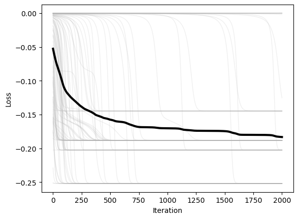

x = np.linspace(-3, 3, 100)
y = np.linspace(-3, 3, 100)
xx, yy = np.meshgrid(x, y)
X = np.array([xx.ravel(), yy.ravel()]).T
Z = loss.loss(X)

plt.figure(figsize=(8, 4))
plt.subplot(1, 2, 1)
plt.scatter(X[:, 0], X[:, 1], c=Z)
plt.plot(*X0.T, '.')
plt.xlim([-3, 3])
plt.ylim([-3, 3])
plt.axis('off')
plt.title('Initial Guesses')

plt.subplot(1, 2, 2)
Xs = np.array(optimizer.Xs)
plt.scatter(X[:, 0], X[:, 1], c=Z)
plt.plot(Xs[0, :, 0], Xs[0, :, 1], '.');
plt.plot(Xs[:, :, 0], Xs[:, :, 1], '-');
plt.plot(Xs[-1, :, 0], Xs[-1, :, 1], '.b', zorder=10);
plt.xlim([-3, 3])
plt.ylim([-3, 3])
plt.axis('off')
plt.title('Trajectories')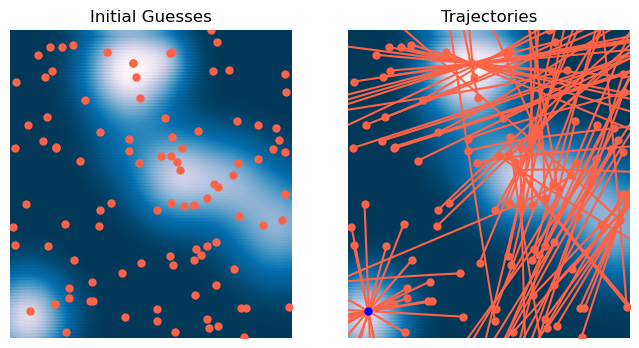

from matplotlib.animation import FuncAnimation
from matplotlib.collections import LineCollection
from IPython.display import HTML

Xs = np.array(optimizer.Xs)[::2][:500]

fig, ax = plt.subplots(figsize=(6, 6))
# ax.scatter(X[:, 0], X[:, 1], c=Z, s=14, zorder=0)
plt.imshow(Z.reshape(100, 100), extent=[-3, 3, -3, 3], origin='lower');
ax.plot(Xs[0, :, 0], Xs[0, :, 1], '.', ms=6, linestyle='None', zorder=1);
curr = ax.scatter([], [], s=20, c='b', zorder=3)
trail = LineCollection([], zorder=2)
ax.add_collection(trail)

ax.set_xlim(-3, 3); ax.set_ylim(-3, 3); ax.axis('off')
plt.margins(0, 0); plt.gca().xaxis.set_major_locator(plt.NullLocator())
plt.gca().yaxis.set_major_locator(plt.NullLocator())

def init():
    curr.set_offsets(np.array([0, 0]))
    trail.set_segments([])
    return (curr, trail)

def update(t):
    # current points
    curr.set_offsets(Xs[t])

    if t > 0:
        segs = []
        # Build one polyline per particle (skip if fewer than 2 points)
        for n in range(Xs.shape[1]):
            path = Xs[:t+1, n, :]  # (k,2)
            if path.shape[0] >= 2:
                segs.append(path)
        trail.set_segments(segs)


    return (curr, trail)

ani = FuncAnimation(fig, update, frames=min(500, Xs.shape[0]),
                    init_func=init, interval=100, blit=True, repeat=True)
html = ani.to_html5_video()
HTML(html)

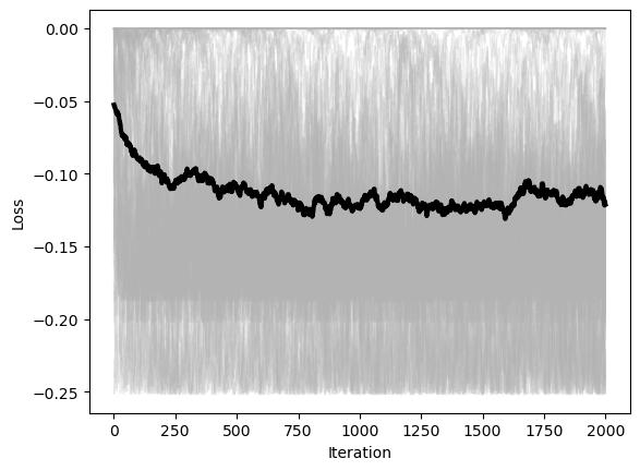
Stochastic Gradient Descent¶

We can also add stochasticity to the gradient descent update rule

\mathbf{x} \leftarrow \mathbf{x} - \eta \nabla \mathcal{L}(\mathbf{x}) + \boldsymbol{\epsilon_t}

(18)

where $\boldsymbol{\epsilon_t} \in \mathbb{R}^D$ is a random noise term

Dynamical interpretation:¶

We can add a time-dependent noise term to our overdamped dynamical system for gradient descent.

\dot{\mathbf{x}} = -\frac{1}{\gamma}\nabla \mathcal{U}(\mathbf{x}) + \boldsymbol{\xi_t}

(19)

Usually we assume that the noise term is a Langevin process, such as the random “kicks” encountered during the Brownian motion of a particle in a fluid. For each component of the vector $\boldsymbol{\epsilon_t}$ ,

\langle \xi_t \xi_s \rangle = 2 \gamma \delta(t-s)

(20)

\langle \xi_t \rangle = 0

(21)

Over discrete times steps, this corresponds the noise vector having a Gaussian distribution with zero mean. We also assume that the different dimensions of the noise force are uncorrelated (the covariance matrix is diagonal).

class StochasticGradientDescent(BaseOptimizer):
    """A Multivariate Gradient Descent Optimizer"""

    def __init__(self, loss, noise, **kwargs):
        super().__init__(loss, **kwargs)
        self.noise = noise

    def update(self, X):
        grad = self.loss.grad(self.X)
        noisy_grad = grad + self.noise * np.random.randn(*grad.shape)
        return X - self.lr * noisy_grad

A Caveat: SGD is different in machine learning.

Our stochastic gradient descent update rule randomly sample a noise vector and then nudges the gradient vector accordingly
The stochastic gradient descent rules often encountered in machine learning models randomly sample a minibatch of training data points. Because the loss landscape in machine learning depends on the dataset, this means that SGD in ML is equivalent to jittering the landscape, not the optimizer state variable. So the dynamics instead have the form

\dot{\mathbf{x}} = -\frac{1}{\gamma}\nabla \mathcal{U}_{\boldsymbol{\theta}}(\mathbf{x})

(22)

where $\boldsymbol{\theta}$ is a random process that describes the parameters of the landscape changing randomly.

In practice, both batch-based SGD gives rise to similar dynamics to a true Langevin process. However, some unique phenomena can occur in ML SGD, such as nonequilibrium behaviors.

optimizer = StochasticGradientDescent(loss, lr=0.1, noise=0.9, max_iter=2000, tol=1e-6, random_state=0, store_history=True)
X0 = 6 * np.random.random(size=(100, 2)) - 3
optimizer.fit(X0.copy())

plt.figure()
plt.plot(optimizer.losses, color=(0.7, 0.7, 0.7), lw=1, alpha=0.2)
plt.plot(np.mean(optimizer.losses, axis=1), 'k', lw=3)
plt.xlabel('Iteration')
plt.ylabel('Loss')

x = np.linspace(-3, 3, 100)
y = np.linspace(-3, 3, 100)
xx, yy = np.meshgrid(x, y)
X = np.array([xx.ravel(), yy.ravel()]).T
Z = loss.loss(X)

plt.figure(figsize=(8, 4))
plt.subplot(1, 2, 1)
plt.scatter(X[:, 0], X[:, 1], c=Z)
plt.plot(*X0.T, '.')
plt.xlim([-3, 3])
plt.ylim([-3, 3])
plt.axis('off')
plt.title('Initial Guesses')

plt.subplot(1, 2, 2)
Xs = np.array(optimizer.Xs)
plt.scatter(X[:, 0], X[:, 1], c=Z)
plt.plot(Xs[0, :, 0], Xs[0, :, 1], '.');
plt.plot(Xs[:, :, 0], Xs[:, :, 1], '-');
plt.plot(Xs[-1, :, 0], Xs[-1, :, 1], '.b', zorder=10);
plt.xlim([-3, 3])
plt.ylim([-3, 3])
plt.axis('off')
plt.title('Trajectories')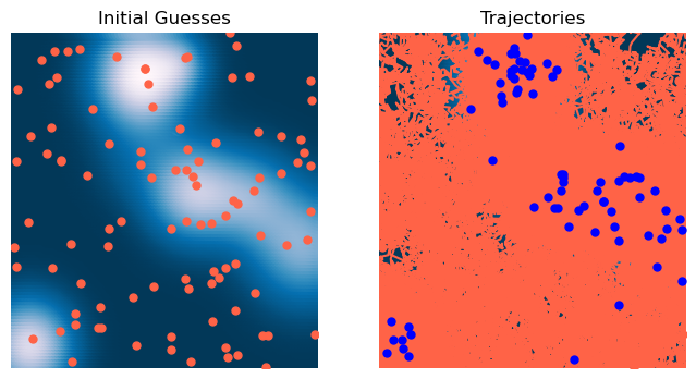

from matplotlib.animation import FuncAnimation
from matplotlib.collections import LineCollection
from IPython.display import HTML

Xs = np.array(optimizer.Xs)[::2][:500]

fig, ax = plt.subplots(figsize=(6, 6))
# ax.scatter(X[:, 0], X[:, 1], c=Z, s=14, zorder=0)
plt.imshow(Z.reshape(100, 100), extent=[-3, 3, -3, 3], origin='lower');
ax.plot(Xs[0, :, 0], Xs[0, :, 1], '.', ms=6, linestyle='None', zorder=1);
curr = ax.scatter([], [], s=20, c='b', zorder=3)
trail = LineCollection([], zorder=2)
ax.add_collection(trail)

ax.set_xlim(-3, 3); ax.set_ylim(-3, 3); ax.axis('off')
plt.margins(0, 0); plt.gca().xaxis.set_major_locator(plt.NullLocator())
plt.gca().yaxis.set_major_locator(plt.NullLocator())

def init():
    curr.set_offsets(np.array([0, 0]))
    trail.set_segments([])
    return (curr, trail)

def update(t):
    # current points
    curr.set_offsets(Xs[t])

    if t > 0:
        segs = []
        # Build one polyline per particle (skip if fewer than 2 points)
        for n in range(Xs.shape[1]):
            path = Xs[:t+1, n, :]  # (k,2)
            if path.shape[0] >= 2:
                segs.append(path)
        trail.set_segments(segs)


    return (curr, trail)

ani = FuncAnimation(fig, update, frames=min(500, Xs.shape[0]),
                    init_func=init, interval=100, blit=True, repeat=True)
html = ani.to_html5_video()
HTML(html)

First-order methods are widely-used for training deep neural networks¶

Stochastic gradient descent remains suprisingly effective in modern settings. Remember that the stochasticity in ML comes from approximating our loss landscape from a subset of the data, not from the noise term in the update rule. Modern optimizers like AdamW, Muon, Adagrad, RMSprop, etc. are all variants of stochastic gradient descent. Many implement forms of momentum by tracking gradients over time, using the gradient history to adapt the learning rate and gradient in various ways.

Second order methods¶

So far, we have only been using methods in which we take the first derivative of the loss function. As we saw in the 1D case, we can converge much faster by using information from the second derivative of the loss function to adjust our learning rate.

For a loss function $\mathcal{L}(\mathbf{x}) \in \mathbb{R}$ computed at location $\mathbf{x} \in \mathbb{R}^d$ , the second derivative is given by the Hessian matrix, $\mathbf{H} = \nabla^2 \mathcal{L}(\mathbf{x}) \in \mathbb{R}^{d \times d}$

Writing this out in matrix form, we have

\mathbf{H} = \begin{bmatrix} \frac{\partial^2 \mathcal{L}(\mathbf{x})}{\partial x_1^2} & \frac{\partial^2 \mathcal{L}(\mathbf{x})}{\partial x_1 \partial x_2} & \cdots & \frac{\partial^2 \mathcal{L}(\mathbf{x})}{\partial x_1 \partial x_d} \\ \frac{\partial^2 \mathcal{L}(\mathbf{x})}{\partial x_2 \partial x_1} & \frac{\partial^2 \mathcal{L}(\mathbf{x})}{\partial x_2^2} & \cdots & \frac{\partial^2 \mathcal{L}(\mathbf{x})}{\partial x_2 \partial x_d} \\ \vdots & \vdots & \ddots & \vdots \\ \frac{\partial^2 \mathcal{L}(\mathbf{x})}{\partial x_d \partial x_1} & \frac{\partial^2 \mathcal{L}(\mathbf{x})}{\partial x_d \partial x_2} & \cdots & \frac{\partial^2 \mathcal{L}(\mathbf{x})}{\partial x_d^2} \end{bmatrix}

(23)

Recalling our intuition from the 1D case, we can see that the Hessian matrix is a measure of how steeply curved the loss function appears at a given point. If the Hessian is positive definite, then the loss function is locally convex, and we can use the second derivative to adjust our learning rate.

The Hessian of the Random Gaussian well landcape¶

Recall that our test landscape is a sum of Gaussian wells,

\mathcal{L} = \sum_{p=1}^P \mathcal{L}_p = -\sum_{p=1}^P A_p \exp\left(-\frac{(\mathbf{x} - \boldsymbol{\mu}_{p})^2}{2\sigma^2}\right)

(24)

where $\mathbf{x} \in \mathbb{R}^d$ is the location in the landscape, $\boldsymbol{\mu}_p \in \mathbb{R}^d$ is the center of the $p$ th well, and $\sigma$ is the width of the well.

The gradient of the loss function is given by

\nabla \mathcal{L} = \sum_{p=1}^P A_p\exp\left(-\frac{(\mathbf{x} - \boldsymbol{\mu}_{p})^2}{2\sigma^2}\right) \frac{(\mathbf{x} - \boldsymbol{\mu}_{p})}{\sigma^2}

(25)

The Hessian matrix is given by

\mathbf{H} = \sum_{p=1}^P A_p \exp\left(-\frac{(\mathbf{x} - \boldsymbol{\mu}_{p})^2}{2\sigma^2}\right) \left(\frac{1}{\sigma^2} \mathbf{I} - \frac{(\mathbf{x} - \boldsymbol{\mu}_{p})(\mathbf{x} - \boldsymbol{\mu}_{p})^T}{\sigma^4}\right)

(26)

Note the order of the last product, which is an outer product and not a contracting inner product. We add this derived implementation of the Hessian matrix to our loss object using subclassing.

class RandomLossLandscapeWithHessian(RandomLossLandscape):
    """
    Subclass of the Random Gaussian Loss Landscape that adds an analytic Hessian calculation
    """

    def __init__(self, **kwargs):
        super().__init__(**kwargs)
        # Everything is passed to the RandomLossLandscape constructor

    def _hessian_gaussian_well(self, X, width=1):
        oprod = np.einsum('ijk,imk->ijmk', X, X) # (n, d, d, 1)
        iden = np.eye(X.shape[1])[None, ..., None] 
        return (-iden + oprod / width**2) / width**2 * self._gaussian_well(X, width)[:, None, None, :]

    def hessian(self, X): 
        return np.einsum('...i,i->...', self._hessian_gaussian_well(X[..., None] - self.locs.T[None, :], self.widths), self.coeffs)

loss = RandomLossLandscapeWithHessian(random_state=0, n_wells=8)

We can look at how the Hessian matrix changes as we move around the landscape. For each point, we compute the Hessian matrix and then plot its scalar condition number. In areas where the Hessian is close to singular, the condition number is large. These indicate regions where the loss landscape is strongly anisotropic, like valleys or ridges between extrema.


x = np.linspace(-3, 3, 100)
y = np.linspace(-3, 3, 100)
xx, yy = np.meshgrid(x, y)
X = np.array([xx.ravel(), yy.ravel()]).T
Z = loss(X) # same as loss.loss(X) because class is callable

plt.figure(figsize=(10, 3))
plt.subplot(1, 3, 1)
plt.scatter(X[:, 0], X[:, 1], c=Z)
plt.plot(xx.ravel()[Z.argmin()], yy.ravel()[Z.argmin()], '*r', markersize=10)
plt.axis('off')

plt.subplot(1, 3, 3)
plt.scatter(X[:, 0], X[:, 1], c=np.log10(np.linalg.cond(loss.hessian(X))))
plt.plot(xx.ravel()[Z.argmin()], yy.ravel()[Z.argmin()], '*r', markersize=10)
plt.axis('off')

plt.subplot(1, 3, 2)
plt.quiver(X[:, 0], X[:, 1], loss.grad(X)[:, 0], loss.grad(X)[:, 1], Z, scale=1e1)
plt.axis('off')

(np.float64(-3.3), np.float64(3.3), np.float64(-3.3), np.float64(3.3))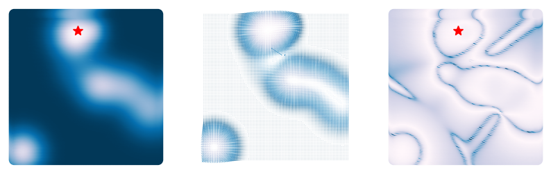

The multivariate Newton’s method¶

Recall that, in one dimension, Newton’s method had the simple form,

x_{t+1} = x_t - \frac{f'(x_t)}{f''(x_t)}

(27)

In higher dimensions, the equivalent of the second derivative is the full $D \times D$ Hessian matrix. The update rule is given by

\mathbf{x} \leftarrow \mathbf{x} - \mathbf{H}^{-1} \nabla \mathcal{L}(\mathbf{x}_t)

(28)

We can interpret this as (1) scaling the size of a gradient descent step by the curvature of the loss function, and (2) rotating the step to align with the eigenvectors of the Hessian matrix. Aligning with the eigenvectors of the Hessian results in straighter paths to the minimum.

We can also add a damping hyperparameter $\alpha$ in the update rule, which slows down the rate of convergence but can help with stability.

\mathbf{x} \leftarrow \alpha \mathbf{x} - (1 - \alpha) \mathbf{H}^{-1} \nabla \mathcal{L}(\mathbf{x}_t)

(29)

class MultivariateNewtonsMethod(BaseOptimizer):
    """
    Optimize a function, subject to the constraint that the solution lies in a convex set.
    """
    def __init__(self, loss, damping=1e-6, armijo_c=1e-4, **kwargs):
        super().__init__(loss, **kwargs)
        self.damping = damping
        self.armijo_c = armijo_c

    @staticmethod
    def _scalar_loss(f):
        """Aggregate per-sample loss to a scalar."""
        f = np.asarray(f)
        return float(np.mean(f))

    def _solve_newton_step(self, hess, grad):
        """Solve H s = g (batched over the first axis) with LM-style damping; 
        avoid explicit inverse."""
        lam = self.damping
        I = np.eye(hess.shape[-1])[None, ...]  # (1,d,d), broadcasts over batch
        for _ in range(6):
            try:
                step = np.linalg.solve(hess + lam * I, grad[..., None])[..., 0]
                return step, lam
            except np.linalg.LinAlgError:
                lam *= 10.0
        # fallback
        step = np.einsum('...ij,...j->...i', np.linalg.pinv(hess + lam * I), grad, optimize=True)
        return step, lam

    def fit(self, X):
        self.X = X
        if self.store_history:
            self.Xs = [self.X.copy()]
            self.losses = [self.loss(X)]

        # f_prev = self._scalar_loss(self.loss(self.X))
        for _ in range(self.max_iter):
            grad = self.loss.grad(self.X)            # (n,d)
            hess = self.loss.hessian(self.X)         # (n,d,d)

            if np.max(np.linalg.norm(grad, axis=1)) < self.tol:
                break
            
            X_new = list()
            ## Iterate over batch dimension. Add a small constant to the Hessian to 
            ## prevent it from being singular.
            for i in range(self.X.shape[0]):
                X_new.append(self.X[i] - self.lr * np.linalg.inv(hess[i] + 1e-12 * np.eye(self.X.shape[1])) @ grad[i])
            X_new = np.array(X_new)

            # step, _ = self._solve_newton_step(hess, grad)  # (n,d)

            # if self.lr is not None and self.lr > 0:
            #     alpha = self.lr
            #     X_new = self.X - alpha * step
            #     f_new = self._scalar_loss(self.loss(X_new))
            # else:
            #     # Armijo backtracking with scalar losses
            #     alpha = 1.0
            #     g2 = float(np.sum(grad * grad))
            #     X_new = self.X - alpha * step
            #     f_new = self._scalar_loss(self.loss(X_new))
            #     rhs = f_prev - self.armijo_c * alpha * g2
            #     while f_new > rhs and alpha > 1e-8:
            #         alpha *= 0.5
            
            #         X_new = self.X - alpha * step
            #         f_new = self._scalar_loss(self.loss(X_new))
            #         rhs = f_prev - self.armijo_c * alpha * g2

            self.X = X_new
            # f_prev = f_new

            if self.store_history:
                self.Xs.append(self.X.copy())
                self.losses.append(self.loss(self.X))

        return self

optimizer = MultivariateNewtonsMethod(loss, max_iter=1000, tol=1e-6, random_state=0, store_history=True)
X0 = 6 * np.random.random(size=(100, 2)) - 3
optimizer.fit(X0.copy())

plt.figure()
plt.plot(np.array(optimizer.losses), color=(0.7, 0.7, 0.7), lw=1, alpha=0.2)
plt.plot(np.mean(np.array(optimizer.losses), axis=1), 'k', lw=3)
plt.xlabel('Iteration')
plt.ylabel('Loss')

x = np.linspace(-3, 3, 100)
y = np.linspace(-3, 3, 100)
xx, yy = np.meshgrid(x, y)
X = np.array([xx.ravel(), yy.ravel()]).T
Z = loss.loss(X)

plt.figure(figsize=(8, 4))
plt.subplot(1, 2, 1)
plt.scatter(X[:, 0], X[:, 1], c=Z)
plt.plot(*X0.T, '.')
plt.xlim([-3, 3])
plt.ylim([-3, 3])
plt.axis('off')
plt.title('Initial Guesses')

plt.subplot(1, 2, 2)
Xs = np.array(optimizer.Xs)
plt.scatter(X[:, 0], X[:, 1], c=Z)
plt.plot(Xs[0, :, 0], Xs[0, :, 1], '.');
plt.plot(Xs[:, :, 0], Xs[:, :, 1], '-');
plt.plot(Xs[-1, :, 0], Xs[-1, :, 1], '.b', zorder=10);
plt.xlim([-3, 3])
plt.ylim([-3, 3])
plt.axis('off')
plt.title('Trajectories')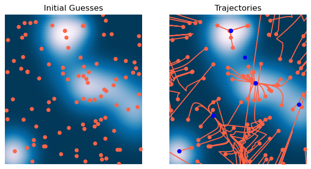

from matplotlib.animation import FuncAnimation
from matplotlib.collections import LineCollection
from IPython.display import HTML

Xs = np.array(optimizer.Xs)[::2][:500]

fig, ax = plt.subplots(figsize=(6, 6))
# ax.scatter(X[:, 0], X[:, 1], c=Z, s=14, zorder=0)
plt.imshow(Z.reshape(100, 100), extent=[-3, 3, -3, 3], origin='lower');
ax.plot(Xs[0, :, 0], Xs[0, :, 1], '.', ms=6, linestyle='None', zorder=1);
curr = ax.scatter([], [], s=20, c='b', zorder=3)
trail = LineCollection([], zorder=2)
ax.add_collection(trail)

ax.set_xlim(-3, 3); ax.set_ylim(-3, 3); ax.axis('off')
plt.margins(0, 0); plt.gca().xaxis.set_major_locator(plt.NullLocator())
plt.gca().yaxis.set_major_locator(plt.NullLocator())

def init():
    curr.set_offsets(np.array([0, 0]))
    trail.set_segments([])
    return (curr, trail)

def update(t):
    # current points
    curr.set_offsets(Xs[t])

    if t > 0:
        segs = []
        # Build one polyline per particle (skip if fewer than 2 points)
        for n in range(Xs.shape[1]):
            path = Xs[:t+1, n, :]  # (k,2)
            if path.shape[0] >= 2:
                segs.append(path)
        trail.set_segments(segs)


    return (curr, trail)

ani = FuncAnimation(fig, update, frames=min(500, Xs.shape[0]),
                    init_func=init, interval=100, blit=True, repeat=True)
html = ani.to_html5_video()
HTML(html)

The results are underwhelming¶

The Newton method underperforms here because our objective function is non-convex, so convergence is not guaranteed. Notice that points close to wells quickly converge; it’s the points in between wells that have trouble. That’s because these are regions in the landscape that don’t locally resemble a concave harmonic potential. For example, a region near a local maximum resembles a convex potential, while other regions might resemble saddles with mixtures of uphill and downhill directions. Another way of saying this is that Newton’s method requires the Hessian to be positive definite

We can understand this better by looking at the eigenvalues of the Hessian matrix. Since the Hessian is a $D \times D$ matrix, it has $D$ eigenvalues. The case where the Hessian is positive definite is when all of the eigenvalues are positive, while the case where the Hessian is negative definite (and thus the landscape resembles a local maximum) is when all of the eigenvalues are negative. Saddle-like regions have mixed signs in their eigenvalues.

To understand this better, for each point in the landscape, we can calculate the sum of the signs of the eigenvalues of the Hessian matrix. We can think of this as measuring the sign of the trace of the Hessian at that point.

def eigval_signs(A):
    esign = np.sign(np.linalg.eigvals(A))
    return np.sum(esign, axis=1)

plt.figure(figsize=(4, 4))
plt.scatter(X[:, 0], X[:, 1], c=eigval_signs(loss.hessian(X)), cmap="coolwarm")
# plt.plot(xx.ravel()[Z.argmin()], yy.ravel()[Z.argmin()], '*r', markersize=10, c="coolwarm")
plt.axis('off')

(np.float64(-3.3), np.float64(3.3), np.float64(-3.3), np.float64(3.3))

While Newton’s method is not guaranteed to converge for non-convex functions, quasi-Newton methods inherit some of the benefits of Newton’s method, while gaining the ability to handle non-convex functions. Instead of building and inverting the full $D \times D$ Hessian matrix, quasi-Newton methods use an approximation to the inverse Hessian matrix, which is updated at each step.

The spectrum of the Hessian¶

The eigenvalues of the Hessian matrix are a measure of how steeply the loss function changes in each direction. For a harmonic potential, they give us the stiffness of the potential in each direction. We can Taylor expand the potential around a given point $\mathbf{x}$ , relative to a nearby point $\mathbf{x}'$

\mathcal{L}(\mathbf{x}) \approx \mathcal{L}(\mathbf{x'}) + \nabla \mathcal{L}(\mathbf{x'})^T (\mathbf{x} - \mathbf{x'}) + \frac{1}{2} (\mathbf{x} - \mathbf{x'})^T \mathbf{H}(\mathbf{x'}) (\mathbf{x} - \mathbf{x'}) + ...

(30)

where we assume that $\mathbf{x} - \mathbf{x'}$ is a small displacement. If $\mathbf{x} - \mathbf{x'}$ is aligns with one of the eigenvector axes of a multivariate harmonic potential, then the second term in the Taylor expansion is directly proportional to the eigenvalue associated with that direction.

Because different directions in a multivariate potential have different stiffnesses, the Hessian has distinct eigenvalues, so the relative size of the second term in the Taylor expansion depends on the direction of the displacement $\mathbf{x} - \mathbf{x'}$ . For very oblong potentials, the difference along various directions can be dramatic.

To understand this effect, we can look at how the Hessian eigenvalues vary at different points in the potential.

plt.figure(figsize=(10, 3))
plt.subplot(1, 3, 1)
plt.scatter(X[:, 0], X[:, 1], c=Z)
# plt.plot(xx.ravel()[Z.argmin()], yy.ravel()[Z.argmin()], '*r', markersize=10)
# plt.axis('off')

plt.plot(2, 0, '*g', markersize=10)
print(np.linalg.eigh(loss.hessian(np.array([2, 0]))).eigenvalues)

plt.plot(0, 2, '*r', markersize=10)
print(np.linalg.eigh(loss.hessian(np.array([0, 2]))).eigenvalues)

plt.plot(-2, 0, '*y', markersize=10)
print(np.linalg.eigh(loss.hessian(np.array([-2, 0]))).eigenvalues)

[[0.09982855 0.19946949]]
[[0.16560671 0.19997077]]
[[-0.00161091  0.0002924 ]]

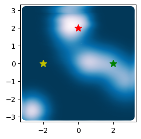
We can the absolute value of the eigenvalues tells us how flat the potential appears along the orthogonal directions associated with the largest and smallest eigenvalues. For the point in the flat region (yellow star), both eigenvalues are small, because the potential is very flat in all directions. For the point near the isolated global minimum (red star), both eigenvalues are large, indicating a very steep region that is nearly isotropic. For the point in the valley connecting the two minima (green star), the largest eigenvalue is small, because the potential is very flat in the direction of the valley, while the smallest eigenvalue is large, because the potential is steep perpendicular to the valley.

We can quantify imbalance among different directions using the condition number, which can be calculated as the ratio of the largest to smallest eigenvalues:

\kappa (H)={\frac {\left|\lambda _{\text{max}}(H)\right|}{\left|\lambda _{\text{min}}(H)\right|}},

(31)

We can think of the valley as a low-dimensional manifold embedded in the high-dimensional optimization space. The dynamics of the optimizer slow down in this region, and we expect that the condition number will be high here.

Adaptive learning rates¶

Optimally, we’d have a separate learning rate for each direction in space, but this becomes computationally expensive in high dimensions. Instead, we can use the condition number to adapt the learning rate.

\mathbf{x} \leftarrow \mathbf{x} - \frac{\eta}{\kappa(\mathbf{H}) + \epsilon} \nabla \mathcal{L}(\mathbf{x})

(32)

where $\eta$ is the initial learning rate, $\kappa(\mathbf{H})$ is the condition number of the Hessian matrix, and $\epsilon$ is a small constant to prevent division by zero.

Another option is to adjust learning rate based only the largest Hessian eigenvalue (we can use the power method to find this quickly in $O(D^2)$ operations, without having to find the full spectrum ( $O(D^3)$ ) or invert the Hessian matrix ( $O(D^3)$ ))

\mathbf{x} \leftarrow \mathbf{x} - \frac{\eta}{\lambda_{\text{max}}} \nabla \mathcal{L}(\mathbf{x})

(33)

where $\lambda_{\text{max}}$ is the largest eigenvalue of the Hessian matrix. We could also adjust the learning rate based on the sum of the largest and smallest eigenvalues of the Hessian matrix.

\mathbf{x} \leftarrow \mathbf{x} - \frac{\eta}{|\lambda_{\text{max}|} + |\lambda_{\text{min}}|} \nabla \mathcal{L}(\mathbf{x})

(34)

we can usually find the largest eigenvalue quickly using the power method, and the smallest eigenvalue using another iterative method, inverse iteration.

class GradientDescentAdaptive(BaseOptimizer):
    """
    Optimize a function, subject to the constraint that the solution lies in a convex set.
    """
    
    def __init__(self, loss, **kwargs):
        super().__init__(loss, **kwargs)
        self.scale_history = []

    def update(self, X):
        grad = self.loss.grad(self.X)
        hess = self.loss.hessian(self.X) #+ 1e-12 * np.eye(self.X.shape[1])[None, ...]

        ## Scale by the largest eigenvalue of the Hessian matrix.
        # scale = np.abs(np.linalg.eigh(hess)[0][-1]) 
        
        scale = 1 / (np.linalg.cond(hess)[:, None] + 1e-12)
        
        ## Recall that the condition number scales with the size of a matrix, so we 
        # correct for this by dividing by the number of dimensions.
        # scale = scale / (hess.shape[1] * 10)
        if self.store_history:
            self.scale_history.append(scale)
        return X - self.lr * grad / scale

optimizer = GradientDescentAdaptive(loss, lr=1e-2, max_iter=2000, tol=1e-6, random_state=0, store_history=True)
X0 = 6 * np.random.random(size=(100, 2)) - 3
optimizer.fit(X0.copy())

plt.figure()
plt.plot(optimizer.losses, color=(0.7, 0.7, 0.7), lw=1, alpha=0.2)
plt.plot(np.mean(optimizer.losses, axis=1), 'k', lw=3)
plt.xlabel('Iteration')
plt.ylabel('Loss')

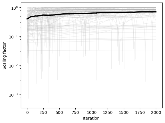
plt.figure()
plt.semilogy(np.array(optimizer.scale_history).squeeze(), color=(0.7, 0.7, 0.7), lw=1, alpha=0.2)
plt.semilogy(np.mean(np.array(optimizer.scale_history), axis=1), 'k', lw=3)
plt.xlabel('Iteration')
plt.ylabel('Scaling factor')

x = np.linspace(-3, 3, 100)
y = np.linspace(-3, 3, 100)
xx, yy = np.meshgrid(x, y)
X = np.array([xx.ravel(), yy.ravel()]).T
Z = loss.loss(X)

plt.figure(figsize=(10, 5))
plt.subplot(1, 2, 1)
plt.scatter(X[:, 0], X[:, 1], c=Z)
plt.plot(*X0.T, '.')
plt.xlim([-3, 3])
plt.ylim([-3, 3])
plt.axis('off')
plt.title('Initial Guesses')

plt.subplot(1, 2, 2)
Xs = np.array(optimizer.Xs)
plt.scatter(X[:, 0], X[:, 1], c=Z, zorder=-2)
plt.plot(Xs[0, :, 0], Xs[0, :, 1], '.');
plt.plot(Xs[:, :, 0], Xs[:, :, 1], zorder=-1);
plt.plot(Xs[-1, :, 0], Xs[-1, :, 1], '.r', markersize=10);
plt.xlim([-3, 3])
plt.ylim([-3, 3])
plt.axis('off')
plt.title('Final Guesses')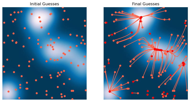

We can see that the condition number is high in flat regions, and so it causes the dynamics to slow down and approximate continuous time dynamics. This means that the condition number damps motion in flat regions. This usually slows down convergence, but it can also help with stability, particularly if we don’t care about the exact location of the minimum, but just want to find any relatively low-loss region.

from matplotlib.animation import FuncAnimation
from matplotlib.collections import LineCollection
from IPython.display import HTML

Xs = np.array(optimizer.Xs)[::2][:500]

fig, ax = plt.subplots(figsize=(6, 6))
# ax.scatter(X[:, 0], X[:, 1], c=Z, s=14, zorder=0)
plt.imshow(Z.reshape(100, 100), extent=[-3, 3, -3, 3], origin='lower');
ax.plot(Xs[0, :, 0], Xs[0, :, 1], '.', ms=6, linestyle='None', zorder=1);
curr = ax.scatter([], [], s=20, c='b', zorder=3)
trail = LineCollection([], zorder=2)
ax.add_collection(trail)

ax.set_xlim(-3, 3); ax.set_ylim(-3, 3); ax.axis('off')
plt.margins(0, 0); plt.gca().xaxis.set_major_locator(plt.NullLocator())
plt.gca().yaxis.set_major_locator(plt.NullLocator())

def init():
    curr.set_offsets(np.array([0, 0]))
    trail.set_segments([])
    return (curr, trail)

def update(t):
    # current points
    curr.set_offsets(Xs[t])

    if t > 0:
        segs = []
        # Build one polyline per particle (skip if fewer than 2 points)
        for n in range(Xs.shape[1]):
            path = Xs[:t+1, n, :]  # (k,2)
            if path.shape[0] >= 2:
                segs.append(path)
        trail.set_segments(segs)


    return (curr, trail)

ani = FuncAnimation(fig, update, frames=min(500, Xs.shape[0]),
                    init_func=init, interval=100, blit=True, repeat=True)
html = ani.to_html5_video()
HTML(html)

Why does this work?¶

The idea behind Newton’s method is to use the second-order Taylor expansion of the loss function to optimally scale the size of steps in each of $D$ dimensions. By using the condition number of the Hessian matrix, we replace the $D$ learning rates with a single scalar, which essentially represents a timescale for the optimization.

Recall that we can usually compute scalar quantities associated with a matrix like the Hessian using less than $O(D^3)$ operations. For example, finding the largest eigenvalue of the Hessian matrix can be done in $O(D^2)$ operations using the power method.

Quasi-Newton methods¶

Creating the Hessian matrix is computationally expensive in high dimensions, requiring at least $O(D^2)$ operations and $O(D^2)$ memory. Inverting it is even worse, requiring ( $O(D^3)$ operations).

We can reduce this cost by approximating the Hessian matrix with a low-rank approximation. Recall that we can write a matrix $H \in \mathbb{R}^{D \times D}$ as $H = Q \Lambda Q^T$ , where $Q \in \mathbb{R}^{D \times D}$ is an orthonormal matrix of eigenvectors and $\Lambda \in \mathbb{R}^{D \times D}$ is a diagonal matrix of eigenvalues. We can also truncate the $Q$ matrices to a low-rank approximation $\tilde{A} \in \mathbb{R}^{D \times D}$ , where $\tilde{A} \approx Q_k \Lambda_k Q_k^T$ , where $Q_k \in \mathbb{R}^{D \times k}$ and $\Lambda_k \in \mathbb{R}^{k \times k}$ are the first $k$ columns of $Q$ and the first $k$ diagonal elements of $\Lambda$ , respectively.

Another popular algorithm is BFGS (the Broyden–Fletcher–Goldfarb–Shanno algorithm). This uses an iterative method to approximate the inverse Hessian matrix directly at each step. Given this approximate inverse Hessian $\tilde{H}_k^{-1}$ , we can compute the step direction using Newton’s method:

\mathbf{x}_{k+1} = \mathbf{x}_k - \tilde{H}_k^{-1} \nabla \mathcal{L}(\mathbf{x}_k)

(35)

Given a history of steps and gradients, we can update the inverse Hessian approximation $\tilde{H}_{k+1}^{-1} \in \mathbb{R}^{D \times D}$ using the following formula:

\tilde{H}_{k+1}^{-1} = \left(I - \frac{\mathbf{v}_k \mathbf{a}_k^T}{\mathbf{a}_k^T \mathbf{v}_k}\right) \tilde{H}_k^{-1} \left(I - \frac{\mathbf{a}_k \mathbf{v}_k^T}{\mathbf{a}_k^T \mathbf{v}_k}\right) + \frac{\mathbf{v}_k \mathbf{v}_k^T}{\mathbf{a}_k^T \mathbf{v}_k}

(36)

where the velocity vector $\mathbf{v}_k = \mathbf{x}_{k+1} - \mathbf{x}_k \in \mathbb{R}^D$ and the acceleration vector $\mathbf{a}_k = \nabla \mathcal{L}(\mathbf{x}_{k+1}) - \nabla \mathcal{L}(\mathbf{x}_k) \in \mathbb{R}^D$ . We initialize the inverse Hessian approximation as the identity matrix, $\tilde{H}_0^{-1} = I$ .

class BFGS(BaseOptimizer):
    def __init__(self, loss, memory=100, **kwargs):
        super().__init__(loss, **kwargs)
        self.memory = memory
        self.grad_hist = []   # ∇f history (per step)
        self.s_hist = []      # x_{k} - x_{k-1} history (per step)
        self.Hk = None        # batched inverse-Hessian approximation, shape (N, D, D)
        self.Hk_history = []  # history of Hk (optional)
        self._prev_X = None   # to form s = x_k - x_{k-1}

    def update(self, X):
        grad = self.loss.grad(X)  # shape (N, D)

        # First step: gradient descent and initialize caches
        if not self.grad_hist:
            self.grad_hist.append(grad)
            self._prev_X = X.copy()
            return X - self.lr * grad

        # Maintain histories (bounded by memory)
        s = X - self._prev_X                      # (N, D)
        y = grad - self.grad_hist[-1]             # (N, D)
        self.s_hist.append(s)
        self.grad_hist.append(grad)
        if len(self.s_hist) > self.memory:
            self.s_hist.pop(0)
        if len(self.grad_hist) > self.memory + 1:  # +1 because grads are one longer than steps
            self.grad_hist.pop(0)

        # Compute / update inverse Hessian (batched)
        Hk = self.get_inverse_hessian_approximation()

        # Step: p_k = - Hk * ∇f(x_k)
        p = np.einsum('nij,nj->ni', Hk, grad)
        self._prev_X = X.copy()
        return X - self.lr * p

    def get_inverse_hessian_approximation(self):
        """
        Batched BFGS update:
            H_{k+1} = (I - rho s y^T) H_k (I - rho y s^T) + rho s s^T,
        where rho = 1 / (y^T s) (done per batch).
        Uses the most recent s and y from history. Initializes H_0 = I.
        """
        # If no step recorded yet, (re)initialize H to identity
        s = self.s_hist[-1]            # (N, D)
        y = self.grad_hist[-1] - self.grad_hist[-2]  # (N, D) (same as above; kept for clarity)
        N, D = s.shape

        # Initialize batched H_0 if needed
        if self.Hk is None or self.Hk.shape != (N, D, D):
            I = np.eye(D)
            self.Hk = np.tile(I, (N, 1, 1)) # Copies along the batch dimension

        H0 = self.Hk
        I = np.eye(D)[None, :, :]                       # (1, D, D) -> broadcast to (N, D, D)

        # ρ_n = 1 / (y_n^T s_n)
        sy = np.einsum('ni,ni->n', s, y)                # (N,)
        rho = 1.0 / (sy + 1e-12)                        # numerical safety
        rho = rho[:, None, None]                        # (N,1,1)

        # Build the batched outer products
        syT = np.einsum('ni,nj->nij', s, y)             # (N, D, D)
        ysT = np.einsum('ni,nj->nij', y, s)             # (N, D, D)
        ssT = np.einsum('ni,nj->nij', s, s)             # (N, D, D)

        # (I - ρ s y^T) and (I - ρ y s^T)
        A = I - rho * syT                               # (N, D, D)
        B = I - rho * ysT                               # (N, D, D)

        # H_{k+1}
        Hk = np.einsum('nij,njk->nik', A, H0)           # A H0
        Hk = np.einsum('nij,njk->nik', Hk, B)           # (A H0) B
        Hk = Hk + rho * ssT                              # + ρ s s^T

        if self.store_history:
            self.Hk_history.append(Hk.copy())

        self.Hk = Hk
        return Hk

loss = RandomLossLandscapeWithHessian(random_state=0, n_wells=8)
optimizer = BFGS(loss, lr=1e-2, max_iter=2000, tol=1e-6, random_state=0, store_history=True)
X0 = 6 * np.random.random(size=(100, 2)) - 3
optimizer.fit(X0.copy())


plt.figure()
plt.plot(optimizer.losses, color=(0.7, 0.7, 0.7), lw=1, alpha=0.2)
plt.plot(np.mean(optimizer.losses, axis=1), 'k', lw=3)
plt.xlabel('Iteration')
plt.ylabel('Loss')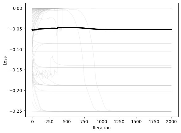

x = np.linspace(-3, 3, 100)
y = np.linspace(-3, 3, 100)
xx, yy = np.meshgrid(x, y)
X = np.array([xx.ravel(), yy.ravel()]).T
Z = loss.loss(X)

plt.figure(figsize=(10, 5))
plt.subplot(1, 2, 1)
plt.scatter(X[:, 0], X[:, 1], c=Z)
plt.plot(*X0.T, '.')
plt.xlim([-3, 3])
plt.ylim([-3, 3])
plt.axis('off')
plt.title('Initial Positions')

plt.subplot(1, 2, 2)
Xs = np.array(optimizer.Xs)
plt.scatter(X[:, 0], X[:, 1], c=Z, zorder=-2)
plt.plot(Xs[0, :, 0], Xs[0, :, 1], '.');
plt.plot(Xs[:, :, 0], Xs[:, :, 1], zorder=-1);
plt.plot(Xs[-1, :, 0], Xs[-1, :, 1], '.r', markersize=10);
plt.xlim([-3, 3])
plt.ylim([-3, 3])
plt.axis('off')
plt.title('Final Positions')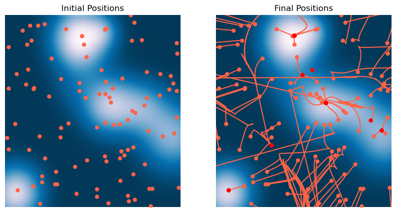

from matplotlib.animation import FuncAnimation
from matplotlib.collections import LineCollection
from IPython.display import HTML

Xs = np.array(optimizer.Xs)[::2][:500]

fig, ax = plt.subplots(figsize=(6, 6))
# ax.scatter(X[:, 0], X[:, 1], c=Z, s=14, zorder=0)
plt.imshow(Z.reshape(100, 100), extent=[-3, 3, -3, 3], origin='lower');
ax.plot(Xs[0, :, 0], Xs[0, :, 1], '.', ms=6, linestyle='None', zorder=1);
curr = ax.scatter([], [], s=20, c='b', zorder=3)
trail = LineCollection([], zorder=2)
ax.add_collection(trail)

ax.set_xlim(-3, 3); ax.set_ylim(-3, 3); ax.axis('off')
plt.margins(0, 0); plt.gca().xaxis.set_major_locator(plt.NullLocator())
plt.gca().yaxis.set_major_locator(plt.NullLocator())

def init():
    curr.set_offsets(np.array([0, 0]))
    trail.set_segments([])
    return (curr, trail)

def update(t):
    # current points
    curr.set_offsets(Xs[t])

    if t > 0:
        segs = []
        # Build one polyline per particle (skip if fewer than 2 points)
        for n in range(Xs.shape[1]):
            path = Xs[:t+1, n, :]  # (k,2)
            if path.shape[0] >= 2:
                segs.append(path)
        trail.set_segments(segs)


    return (curr, trail)

ani = FuncAnimation(fig, update, frames=min(500, Xs.shape[0]),
                    init_func=init, interval=100, blit=True, repeat=True)
html = ani.to_html5_video()
HTML(html)

We can again see that BFGS converges quickly to the minimum only in convex regions of the landscape. Otherwise, it tends to find local maxima and saddle points.

The main limitation of BFGS is that it requires storing an estimate of the $D \times D$ Hessian matrix, which can become memory-intensive in high dimensions. A popular variant of BFGS is L-BFGS (Limited-memory BFGS), which uses a low-rank approximation if the inverse Hessian matrix, reducing memory usage.

The Adam optimizer¶

The Adam optimizer is a popular method for training deep neural networks. It uses the first and second moments of the gradient to adapt the learning rate. It also employs bias corrections to account for the fact that the first and second moments are not unbiased estimates of the true moments. In practice, it uses an exponential moving average to update the first and second moments, resulting in more stable updates.

Each update in Adam consists of the following step:

\mathbf{x}_{t+1} = \mathbf{x}_t - \eta \frac{\tilde{\mathbf{m}}_t}{\sqrt{\tilde{\mathbf{v}}_t} + \epsilon}

(37)

where $\tilde{\mathbf{m}}_t$ and $\tilde{\mathbf{v}}_t$ are the bias-corrected first and second moments of the gradient, respectively, and $\epsilon$ is a small constant to prevent division by zero.

The first and second moments are computed as follows:

\mathbf{m}_t = \beta_1 \mathbf{m}_{t-1} + (1 - \beta_1) \nabla \mathcal{L}(\mathbf{x}_t)

(38)

\mathbf{v}_t = \beta_2 \mathbf{v}_{t-1} + (1 - \beta_2) \nabla \mathcal{L}(\mathbf{x}_t)^2

(39)

where $\beta_1$ and $\beta_2$ are hyperparameters that control the decay rate of the first and second moments, respectively, and $\mathbf{g}_t$ is the gradient at time $t$ . We can see that the first moment is a weighted average of the previous first moment and the current gradient, and the second moment is a weighted average of the previous second moment and the current gradient squared. So the first moment is a kind of moving average of the gradient, and the second moment is a moving average of the gradient squared.

However, this calculation introduces a bias in the estimates of the first and second moments. This is because the first and second moments are initialized to zero, and so the early values of the first and second moments are more heavily weighted by the initial values. We can correct for this bias by using the following bias correction terms:

\tilde{\mathbf{m}}_t = \frac{\mathbf{m}_t}{1 - \beta_1^t}

(40)

\tilde{\mathbf{v}}_t = \frac{\mathbf{v}_t}{1 - \beta_2^t}

(41)

where $t$ is the time step. This corresponds to an exponential moving average of the first and second moments, which weights the early values more heavily.

class AdamOptimizer(BaseOptimizer):
    """
    Minimal Adam optimizer.

    """
    def __init__(self, loss, beta1=0.9, beta2=0.999, eps=1e-8, **kwargs):
        super().__init__(loss, **kwargs)
        self.beta1 = beta1
        self.beta2 = beta2
        self.eps = eps
        self.m = None
        self.v = None
        self.t = 0

    def update(self, X):
        # Lazy state initialization (handles shape (n_dim,) or (n_batch, n_dim))
        if self.m is None or self.v is None:
            self.m = np.zeros_like(X, dtype=float)
            self.v = np.zeros_like(X, dtype=float)
            self.t = 0

        self.t += 1
        g = self.loss.grad(X)

        # Exponential moving averages
        self.m = self.beta1 * self.m + (1.0 - self.beta1) * g
        self.v = self.beta2 * self.v + (1.0 - self.beta2) * (g * g)

        # Bias corrections based on exponential moving averages
        m_hat = self.m / (1.0 - self.beta1 ** self.t)
        v_hat = self.v / (1.0 - self.beta2 ** self.t)

        # Parameter update
        X_new = X - self.lr * m_hat / (np.sqrt(v_hat) + self.eps)
        # X_new = X - self.lr * self.loss.grad(X)
        return X_new

optimizer = AdamOptimizer(loss, lr=0.1, max_iter=2000, tol=1e-6, random_state=0, store_history=True)
X0 = 6 * np.random.random(size=(100, 2)) - 3
optimizer.fit(X0.copy())

plt.figure()
plt.plot(optimizer.losses, color=(0.7, 0.7, 0.7), lw=1, alpha=0.2)
plt.plot(np.mean(optimizer.losses, axis=1), 'k', lw=3)
plt.xlabel('Iteration')
plt.ylabel('Loss')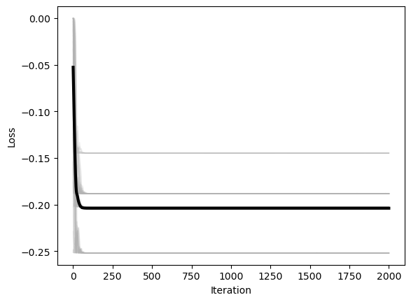

x = np.linspace(-3, 3, 100)
y = np.linspace(-3, 3, 100)
xx, yy = np.meshgrid(x, y)
X = np.array([xx.ravel(), yy.ravel()]).T
Z = loss.loss(X)

plt.figure(figsize=(10, 5))
plt.subplot(1, 2, 1)
plt.scatter(X[:, 0], X[:, 1], c=Z)
plt.plot(*X0.T, '.')
plt.xlim([-3, 3])
plt.ylim([-3, 3])
plt.axis('off')
plt.title('Initial Positions')

plt.subplot(1, 2, 2)
Xs = np.array(optimizer.Xs)
plt.scatter(X[:, 0], X[:, 1], c=Z, zorder=-2)
plt.plot(Xs[0, :, 0], Xs[0, :, 1], '.');
plt.plot(Xs[:, :, 0], Xs[:, :, 1], zorder=-1);
plt.plot(Xs[-1, :, 0], Xs[-1, :, 1], '.r', markersize=10);
plt.xlim([-3, 3])
plt.ylim([-3, 3])
plt.axis('off')
plt.title('Final Positions')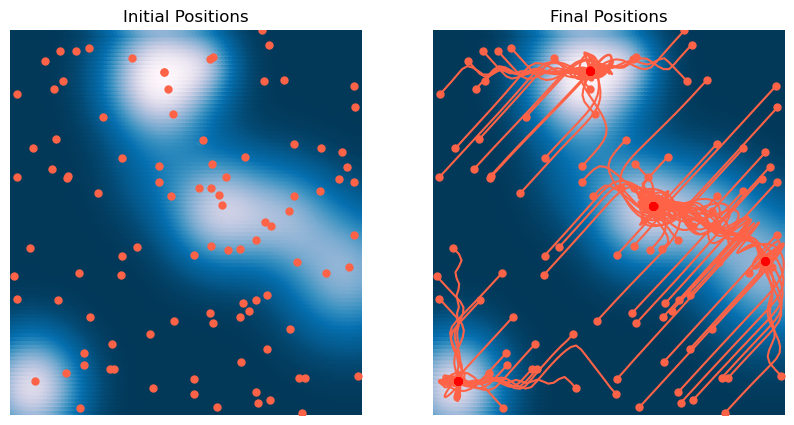

from matplotlib.animation import FuncAnimation
from matplotlib.collections import LineCollection
from IPython.display import HTML

Xs = np.array(optimizer.Xs)[::2][:500]

fig, ax = plt.subplots(figsize=(6, 6))
# ax.scatter(X[:, 0], X[:, 1], c=Z, s=14, zorder=0)
plt.imshow(Z.reshape(100, 100), extent=[-3, 3, -3, 3], origin='lower');
ax.plot(Xs[0, :, 0], Xs[0, :, 1], '.', ms=6, linestyle='None', zorder=1);
curr = ax.scatter([], [], s=20, c='b', zorder=3)
trail = LineCollection([], zorder=2)
ax.add_collection(trail)

ax.set_xlim(-3, 3); ax.set_ylim(-3, 3); ax.axis('off')
plt.margins(0, 0); plt.gca().xaxis.set_major_locator(plt.NullLocator())
plt.gca().yaxis.set_major_locator(plt.NullLocator())

def init():
    curr.set_offsets(np.array([0, 0]))
    trail.set_segments([])
    return (curr, trail)

def update(t):
    # current points
    curr.set_offsets(Xs[t])

    if t > 0:
        segs = []
        # Build one polyline per particle (skip if fewer than 2 points)
        for n in range(Xs.shape[1]):
            path = Xs[:t+1, n, :]  # (k,2)
            if path.shape[0] >= 2:
                segs.append(path)
        trail.set_segments(segs)


    return (curr, trail)

ani = FuncAnimation(fig, update, frames=min(500, Xs.shape[0]),
                    init_func=init, interval=100, blit=True, repeat=True)
html = ani.to_html5_video()
HTML(html)

A bakeoff: Which method is the best?¶

We can compare the performance of the different methods we’ve seen so far. We compute two metrics: the final loss value, and the total amount of walltime required to reach that loss value. A more accurate measure of performance might count individual operations and memory usage, rather than aggregate walltime, but the walltime should give us an idea of the tradeoffs involved.

import time

## Set up our loss function and initial conditions
loss = RandomLossLandscapeWithHessian(random_state=0, n_wells=8)
X0 = 6 * np.random.random(size=(500, 2)) - 3

## Set our optimizers and hyperparameters
optimizer_kwargs = {"max_iter": 5000, "lr": 0.1, "tol": 1e-6, "random_state": 0, "store_history": True}
optimizer_list = [
    GradientDescent(loss, **optimizer_kwargs),
    AdamOptimizer(loss, **optimizer_kwargs),
    GradientDescentMomentum(loss, **optimizer_kwargs),
    StochasticGradientDescent(loss, noise=0.2, **optimizer_kwargs),
    MultivariateNewtonsMethod(loss, **optimizer_kwargs),
    GradientDescentAdaptive(loss, **optimizer_kwargs),
    BFGS(loss, **optimizer_kwargs),
]

all_losses = []
all_walltimes = []

for optimizer in optimizer_list:
    
    start_time = time.time()
    optimizer.fit(X0.copy())
    stop_time = time.time()

    final_loss = np.mean(optimizer.losses, axis=1)[-1]
    
    all_losses.append(final_loss)
    all_walltimes.append(stop_time - start_time)
all_losses = np.array(all_losses)
all_walltimes = np.array(all_walltimes)
optimizer_names = np.array([type(o).__name__ for o in optimizer_list])

plt.figure(figsize=(7, 7))
sorted_losses = np.argsort(all_losses)
plt.subplot(2, 1, 1)
plt.barh(optimizer_names[sorted_losses], all_losses[sorted_losses])
plt.title('Final Loss')

plt.subplot(2, 1, 2)
sorted_times = np.argsort(all_walltimes)
plt.barh(optimizer_names[sorted_times], all_walltimes[sorted_times])
plt.title('Wall Time')

plt.figure(figsize=(5, 5))
plt.scatter(all_losses, all_walltimes)
## label optimizers
for i in range(len(optimizer_names)):
    plt.annotate(optimizer_names[i], (all_losses[i], all_walltimes[i]))
plt.xlabel('Final Loss')
plt.ylabel('Wall Time')

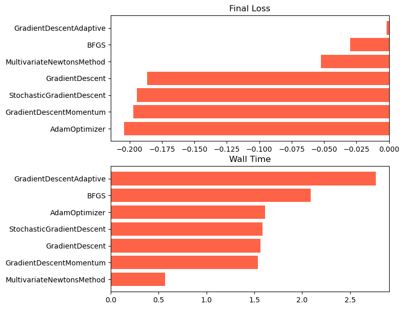
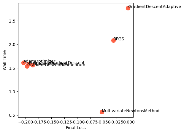
We can see that, for our non-convex two-dimensional landscape, the lightweight gradient-descent methods are the fastest and most accurate. Adam is the second fastest, and the most accurate overall. However, we expect that our results might change with different hyperparameters, on landscapes with rougher curvature, more local minima or saddle points, or higher dimensionality.

What if we can’t compute the derivatives analytically?¶

All of our optimization methods required us to analytically compute the gradient and Hessian matrix. We did this analytically for the random Gaussian loss landscape, but this is not always feasible for arbitrary landscapes, like the loss functions of deep neural networks, which consist of many nonlinear transformations of the input.

One option is to use finite-difference derivatives, which approximate the gradient and Hessian matrix by taking an initial state vector $\mathbf{x}$ and estimating how $\mathcal{L}(\mathbf{x})$ changes when we perturb $\mathbf{x}$ by a small amount in each of the $D$ dimensions. However, the cost of this approach is $O(D)$ operations to find the gradient, and $O(D^2)$ operations to find the Hessian matrix.

There’s another way to compute derivatives that is both exact and fast in high dimensions, called automatic differentiation. Conceptually, when we compute our random Gaussian landscape, we build a series of matrices and then multiply and contract them to obtain a final scalar loss. In automatic differentiation, we store the results of these intermediate calculations when we first compute the loss, a step known as the forward pass. Then, in order to compute the gradient, we can combine these intermediate values in a different order, a step known as the backward pass. This is a consequence of the chain rule for derivatives.

References¶

Maibach, D., Brandenberger, R., Crichton, D., & Refregier, A. (2021). Extracting the signal of cosmic string wakes from 21-cm observations. Physical Review D, 104(12). 10.1103/physrevd.104.123535

Chapters

Lagrangian Duality and constrained optimization

Chapters

Optimization under constraints