Preamble: Run the cells below to import the necessary Python packages
Open this notebook in Google Colab: 
## Preamble / required packages
import numpy as np
np.random.seed(0)

## Import local plotting functions and in-notebook displazooy functions
import matplotlib.pyplot as plt
from IPython.display import Image, display
%matplotlib inline

import warnings
## Comment this out to activate warnings
warnings.filterwarnings('ignore')
Is there anything linear models can’t do?
We previously saw that regularized linear models can be surprisingly effective for supervised learning tasks like forecasting, regression, and even classification. In unsupervised learning, PCA and its variants can be thought of as linear models as well. Given how successful linear models are, we wonder whether there are any problems that are fundamentally beyond the capabilities of linear models. To examine this question, we will consider a simple classification problem consisting of only four datapoints, with two features and two labels.
## AND dataset for training
X = np.array([[0.0, 0], [0, 1], [1, 0], [1, 1]])
y = np.array([0, 0, 0.0, 1.0])

print("Training data has shape: ", X.shape)
print("Target targets have shape: ", y.shape)

## Plot the AND dataset
plt.figure(figsize=(5, 5))
plt.scatter(X[:, 0], X[:, 1], c=y, cmap=plt.cm.coolwarm, s=500)
plt.xlabel("X Feature 1")
plt.ylabel("X Feature 2")
plt.colorbar(label="Target")
Training data has shape: (4, 2)
Target targets have shape: (4,)
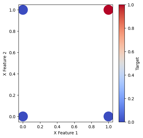
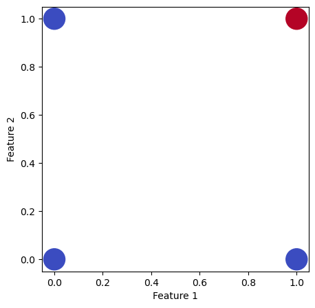
This particular dataset is the AND dataset, because the label is 1 if and only if both features are 1. Since there are discrete-valued labels for each data point, we can think of this as a classification problem. We will now try fitting a linear model to this dataset, using the LogisticRegression class from sklearn.
## train logistic regression model
from sklearn.linear_model import LogisticRegression
model = LogisticRegression(penalty='none')
model.fit(X, y)
yhat = model.predict(X)

print("Predicted labels have shape: ", yhat.shape)
print("Train accuracy: ", np.mean(yhat == y))

plt.figure(figsize=(5, 5))
plt.scatter(X[:, 0], X[:, 1], c=yhat, cmap=plt.cm.coolwarm, s=500)
plt.xlabel("Feature 1")
plt.ylabel("Feature 2")

print(yhat)
Predicted labels have shape: (4,)
Train accuracy: 1.0
[0. 0. 0. 1.]
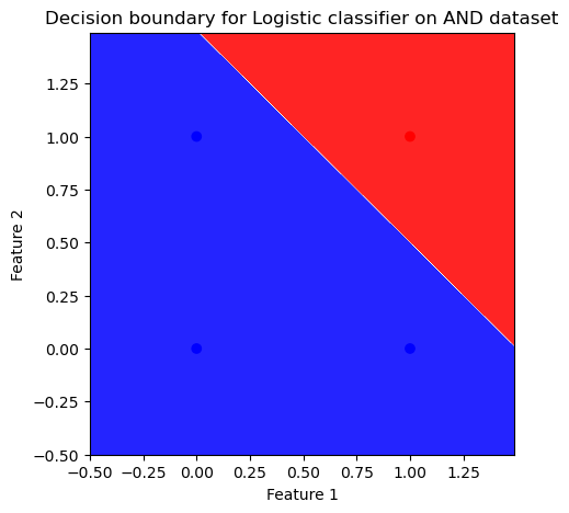
Decision boundaries
In the above plot, we visualized the predicted labels specifically for the training datapoints. However, in principle the training features can have any values in the feature space, and so we can construct a testing dataset spanning the domain of the feature space. That can allow us to determine exactly which combinations of the two inputs lead to a certain predicted label. In trained classification models, labelling each point in this domain reveals the decision boundary of the model.
## plot decision boundary
def plot_decision_boundary(X, y, clf):
    """
    Plot the decision boundary of a trained classifier clf

    Args:
        X (numpy.ndarray): Input data
        y (numpy.ndarray): Input labels
        clf (sklearn.base.BaseEstimator): Trained classifier

    Returns:
        None
    """
    # Set min and max values and give it some padding
    x_min, x_max = X[:, 0].min() - .5, X[:, 0].max() + .5
    y_min, y_max = X[:, 1].min() - .5, X[:, 1].max() + .5
    h = 0.01

    # Generate a grid of points with distance h between them
    xx, yy = np.meshgrid(np.arange(x_min, x_max, h), np.arange(y_min, y_max, h))

    # Predict the function value for the whole gid
    Z = clf.predict(np.c_[xx.ravel(), yy.ravel()])

    # Put the result into a color plot
    Z = Z.reshape(xx.shape)

    # Plot the contour and training examples
    plt.contourf(xx, yy, Z, cmap='bwr')
    plt.scatter(X[:, 0], X[:, 1], c=y, cmap='bwr')

plt.figure(figsize=(5, 5))
plot_decision_boundary(X, y, model)
plt.xlabel("Feature 1")
plt.ylabel("Feature 2")
plt.title("Decision boundary for Logistic classifier on AND dataset")
Questions
Why is the decision boundary a straight line?
What might influence the location and slope of the decision boundary?
The XOR dataset
We can now do the exact same analysis using a different dataset consisting of only four datapoints, with two features and two labels.
## XOR dataset for training
X = np.array([[0, 0], [0, 1], [1, 0], [1, 1]])
y = np.array([0, 1.0, 1.0, 0.0])

## Plot the XOR dataset
plt.figure(figsize=(5, 5))
plt.scatter(X[:, 0], X[:, 1], c=y, cmap=plt.cm.coolwarm, s=500)
plt.xlabel("Feature 1")
plt.ylabel("Feature 2")


print(X.shape)
print(y.shape)
(4, 2)
(4,)
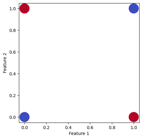
This particular dataset is the XOR dataset, because the label is 1 if and only if one of the features is 1. Thus the label is 1 exclusively when the two features are different. We will now try fitting a linear model to this dataset, using the same procedure as before.
## train logistic regression model
from sklearn.linear_model import LogisticRegression

## XOR dataset for training
X = np.array([[0, 0], [0, 1], [1, 0], [1, 1]])
y = np.array([0, 1.0, 1.0, 0.0])

model = LogisticRegression(penalty='none')
model.fit(X, y)
yhat = model.predict(X)

print("Predicted labels have shape: ", yhat.shape)
print("Train accuracy: ", np.mean(yhat == y))
Predicted labels have shape: (4,)
Train accuracy: 0.5
# plt.figure()
# plt.scatter(X[:, 0], X[:, 1], c=yhat, cmap=plt.cm.coolwarm, s=500)
# plt.xlabel("Feature 1")
# plt.ylabel("Feature 2")


plt.figure(figsize=(5, 5))
plot_decision_boundary(X, y, model)
plt.xlabel("Feature 1")
plt.ylabel("Feature 2")
plt.title("Decision boundary for Logistic classifier on XOR dataset")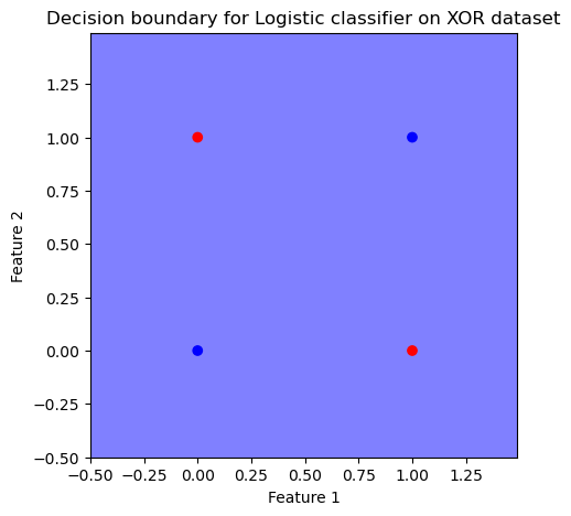
We can see that despite Logistic regression perfectly solving the AND dataset, it does no better than random guessing on the XOR dataset. The decision boundary is nonsensical, implying that the trained model is not internalizing informative features.
This observation is a consequence of XOR being a non-linearly separable problem. Linear models such as logistic regression can only construct hyperplanes, which are insufficient to separate the alternating class structure of XOR. The limitation of linear separability was famously emphasized by Minsky and Papert (1969) in Perceptrons, where they demonstrated that single-layer neural networks cannot represent functions like XOR. This theoretical result highlights the necessity of trainable nonlinear transformations or multiple layers to capture such interactions. Consequently, solving XOR requires either explicit feature engineering (e.g., polynomial terms) or models with nonlinear capacity, such as kernel methods or multi-layer neural networks (MLP), which can form hierarchical representations beyond simple linear decision boundaries.
What is a neural network?
A neural network is a function that takes a vector of inputs and returns a vector of outputs. Unlike a matrix (linear model), a neural network can learn nonlinear transformations of the input. Generally, any function that can be written as a composition of linear transformations and nonlinear functions is a neural network. In any scientific computing problem that can be written as a matrix, one can use a neural network. We can better understand perceptrons by first understanding linear regression, and then generalizing to nonlinear transformations.
Linear regression
A linear model is a function that takes a vector of inputs and returns a scalar output, based on learning a matrix of parameters .
A key advantage of linear models is that they usually have an known optimal solution for the parameters conditioned on a trainingdataset of inputs and outputs . As a result, little hyperparameter tuning or optimization knowledge is needed to train the model. The parameters are also interpretable because they directly quantify the important of each input feature on the output.
Generalized linear regression
A generalized linear model is a function that takes a vector of inputs and returns a scalar output, based on learning a matrix of parameters after applying a nonlinear “link” function .
where is a nonlinear “link” function. For logistic function, .
Like linear models, generalized linear models usually have an known optimal solution for the parameters conditioned on a training dataset of inputs and outputs . They also have interpretable parameters, which can be used to understand the importance of each input feature on the output. However, unlike linear models, the fitting procedure is more complex because the link function is nonlinear.
Multilayer perceptron (a neural network)
A multilayer perceptron (MLP) is a function that takes a vector of inputs and returns a vector of outputs, based on learning a matrix of parameters after applying a nonlinear “link” function .
where is a nonlinear function, and is a matrix of trainable parameters. Unlike generalized linear models, MLPs can learn nonlinear transformations of the input by composing multiple linear transformations with a nonlinear function. The number of trainable parameters in an MLP is the number of entries across all matrices .
## TODO: Add noise to inputs

from sklearn.neural_network import MLPClassifier

model = MLPClassifier(hidden_layer_sizes=(5, 300, 300, 5), activation='tanh', max_iter=1000, random_state=0)

## XOR dataset for training
X = np.array([[0, 0], [0, 1], [1, 0], [1, 1]])
y = np.array([0, 1.0, 1.0, 0.0])

## AND
# X = np.array([[0, 0], [0, 1], [1, 0], [1, 1]])
# y = np.array([0, 0.0, 0.0, 1.0])

model.fit(X, y)
yhat = model.predict(X)

plt.figure(figsize=(5, 5))
plt.scatter(X[:, 0], X[:, 1], c=yhat, cmap=plt.cm.coolwarm, s=500)
plt.xlabel("Feature 1")
plt.ylabel("Feature 2")

plt.figure(figsize=(5, 5))
plot_decision_boundary(X, yhat, model)
plt.xlabel("Feature 1")
plt.ylabel("Feature 2")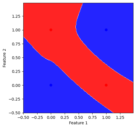
Because multilayer perceptrons learn multiple linear transformations with a nonlinear function, they can learn much more complex transformations of the input. They also typically require more trainable parameters, which allows them to fit more complex functions.
## Read out the weight matrices
# model.coefs_

for layer in model.coefs_:
    print(layer.shape)
(2, 5)
(5, 5)
(5, 1)
What do neural networks do?
Neural networks can learn “arbitrary” nonlinear functions of the data. Cybenko’s theorem states that any continuous function can be approximated by a neural network with a single, sufficiently wide hidden layer. Modern generalizations exist for deep networks with finite width but arbitrary depth. As a result, neural networks are a universal approximator given enough parameters or depth.
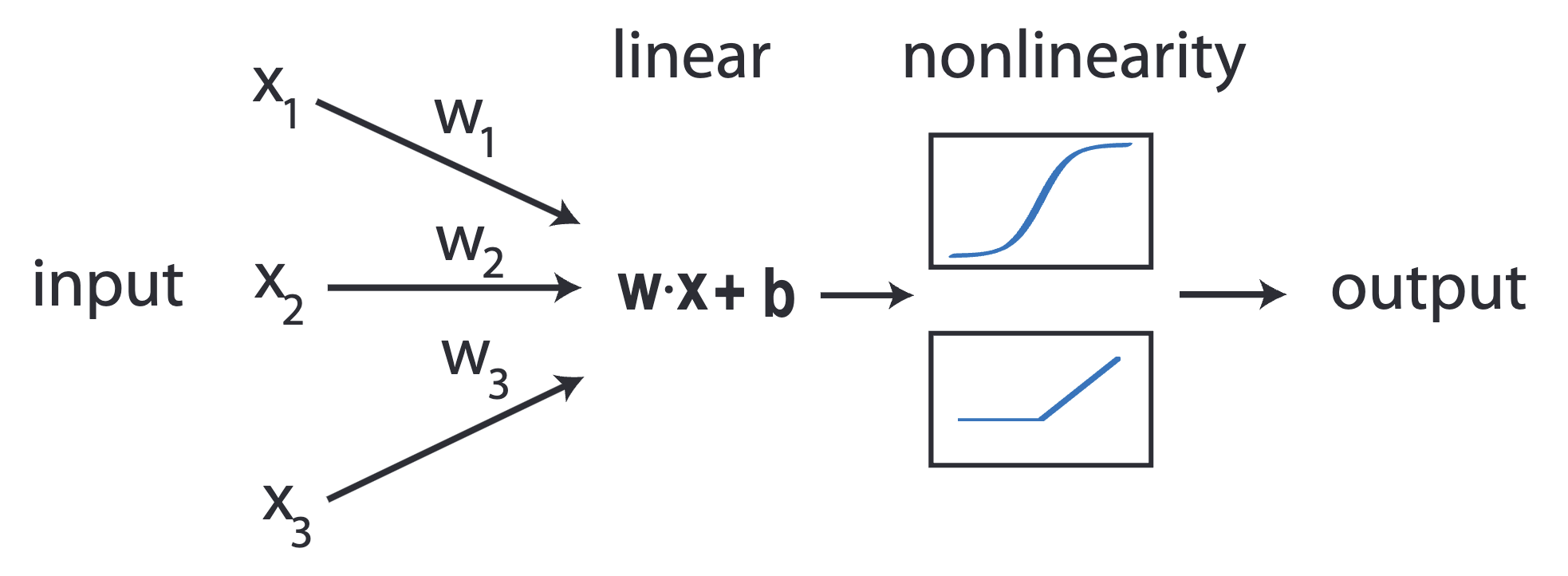
Multilayer perceptron
The most basic neural network is the multilayer perceptron (MLP), which is a composition of matrix multiplications that are each followed by a nonlinear function. The key hyperparameter of an MLP is the depth or number of layers, which controls the depth of the networ, as well as the width of the network, which controls the number of “neurons” (units) per layer. Other common hyperparameters include the choice of activation function and regularization. In multilayer perceptrons, the number of trainable parameters is the number of entries across all matrices. As a result, MLPs are usually overparameterized relative to the number of datapoints in the training set.
Image('../resources/mlp.png')
# https://medium.com/codex/introduction-to-how-an-multilayer-perceptron-works-but-without-complicated-math-a423979897ac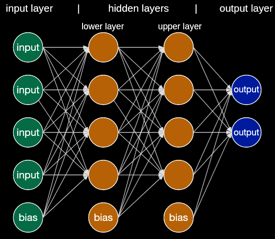
The diagram above is equivalent to writing a function composed of three linear transformations, each followed by a nonlinear function.
where , , . The depth of a network thus determines the total number of compositions of linear transformations, and the width determines the number of linear transformations per layer. We can try writing this function in code, using random (untrained) weights as an illustration
## The code version

def mlp_forward(X):
    theta1 = np.random.random((5, 5))
    theta2 = np.random.random((5, 5))
    theta3 = np.random.random((5, 2))

    h1 = np.tanh(X @ theta1)
    h2 = np.tanh(h1 @ theta2)
    h3 = np.tanh(h2 @ theta3)

    return h3


X = np.random.random((10000, 5))

print("Input shape: ", X.shape)
print("Output shape: ", mlp_forward(X).shape)
Input shape: (10000, 5)
Output shape: (10000, 2)
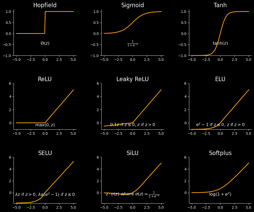
The choice of activation function is itself a hyperparameter
import numpy as np
import matplotlib.pyplot as plt

# Define the activation functions
def hopfield(z):
    return np.where(z >= 0, 1, 0)

def sigmoid(z):
    return 1 / (1 + np.exp(-z))

def tanh(z):
    return np.tanh(z)

def relu(z):
    return np.maximum(0, z)

def leaky_relu(z, alpha=0.1):
    return np.where(z > 0, z, alpha * z)

def elu(z, alpha=1.0):
    return np.where(z > 0, z, alpha * (np.exp(z) - 1))

def selu(z, lambda_=1.0507, alpha=1.67326):
    return np.where(z > 0, lambda_ * z, lambda_ * alpha * (np.exp(z) - 1))

def silu(z):
    return z / (1 + np.exp(-z))

def softplus(z):
    return np.log(1 + np.exp(z))

# Set up the figure and axis
z = np.linspace(-5, 5, 100)
fig, axs = plt.subplots(3, 3, figsize=(12, 9), facecolor='black')
# fig.subplots_adjust(hspace=0.5, wspace=0.4)
fig.subplots_adjust(hspace=0.6, wspace=0.4, top=0.92, bottom=0.08)


# Define titles and functions for each subplot
titles = [
    'Hopfield', 'Sigmoid', 'Tanh', 'ReLU', 'Leaky ReLU', 'ELU',
    'SELU', 'SiLU', 'Softplus'
]
functions = [
    hopfield, sigmoid, tanh, relu, leaky_relu, elu,
    selu, silu, softplus
]
equations = [
    r"$\Theta(z)$",
    r"$\frac{1}{1+e^{-z}}$",
    r"$\tanh(z)$",
    r"$\max(0, z)$",
    r"$0.1z$ if $z \leq 0$, $z$ if $z > 0$",
    r"$e^z - 1$ if $z \leq 0$, $z$ if $z > 0$",
    r"$\lambda z$ if $z > 0$, $\lambda \alpha (e^z - 1)$ if $z \leq 0$",
    r"$z \cdot \sigma(z)$ where $\sigma(z) = \frac{1}{1 + e^{-z}}$",
    r"$\log(1 + e^z)$"
]

# Plot each activation function
for i, (ax, title, func, equation) in enumerate(zip(axs.flat, titles, functions, equations)):
    ax.plot(z, func(z), color='orange', linewidth=2)
    ax.set_title(title, fontsize=16, color='white')
    ax.text(0, -0.5, equation, fontsize=12, color='white', ha='center')
    ax.grid(False)
    ax.set_facecolor('black')
    ax.spines['bottom'].set_color('white')
    ax.spines['left'].set_color('white')
    ax.tick_params(axis='x', colors='white')
    ax.tick_params(axis='y', colors='white')
    if i < 3:
        ax.set_ylim(-1, 1.1)
    elif i < 6:
        ax.set_ylim(-1, 6)
    else:
        ax.set_ylim(-1.8, 6)

plt.show()
A harder classification problem: predicting the Reynolds number of turbulent flows
We can see that there are certain supervised learning problems with sufficiently complex decision boundaries that a neural network is useful. We will extend this idea by considering an intrinsically nonlinear classification problem: predicting the Reynolds number of turbulent flow, giving only observations of the velocity field.
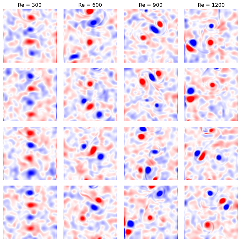
We will use a dataset of videos of wake flows in 2D turbulent flows simulated at different Reynolds numbers. This dataset has spatial noise, which is a common artifact of the PIV algorithm used to extract a velocity field from experimental videos of a flow. We will treat each frame of the video as a single datapoint in our dataset, with a number of features equal to the number of pixels in the frame. We can start by visualizing a few frames of the data from each class, in order to get a sense of how hard classifying the different Reynolds numbers wil be.
## load the turbulence dataset

all_vorticity_fields = list()
all_reynolds_numbers = list()

# Load simulations for different Reynolds numbers
re_vals = [300, 600, 900, 1200]
for re_val in re_vals:

    # Load the two-dimensional velocity field data. Data is stored in a 4D numpy array,
    # where the first dimension is the time index, the second and third dimensions are the
    # x and y coordinates, and the fourth dimension is the velocity components (ux or uv).
    vfield = np.load(
        f"../resources/von_karman_street/vortex_street_velocities_Re_{re_val}_largefile.npz",
        allow_pickle=True
    )

    # Calculate the vorticity, which is the curl of the velocity field
    vort_field = np.diff(vfield, axis=1)[..., :-1, 1] + np.diff(vfield, axis=2)[:, :-1, :, 0]

    # Downsample the dataset
    vort_field = vort_field[::6, -127:, :]

    # Add random experimental noise
    noise_field = np.random.normal(0, 0.02, vort_field.shape)
    ## Gaussian blur the noise field along the x and y axes using scipy.ndimage.gaussian_filter
    from scipy.ndimage import gaussian_filter
    noise_field = gaussian_filter(noise_field, sigma=(0, 4, 4))

    vort_field += noise_field


    all_vorticity_fields.append(vort_field)
    all_reynolds_numbers.extend(re_val * np.ones(vort_field.shape[0]))

all_vorticity_fields = np.vstack(all_vorticity_fields)
all_reynolds_numbers = np.array(all_reynolds_numbers)

print("Vorticity field data has shape: {}".format(all_vorticity_fields.shape))
print("Reynolds number data has shape: {}".format(all_reynolds_numbers.shape))


## Plot 4x4 grid of vorticity fields
fig, ax = plt.subplots(4, 4, figsize=(8, 8))
for i in range(4):
    re_val = re_vals[i]
    for j in range(4):
        ax[j, i].imshow(
            all_vorticity_fields[all_reynolds_numbers == re_val][150 * j],
            cmap='bwr',
            vmin=-0.01, vmax=0.01
        )
        ax[j, i].axis('off')
        if j == 0:
            ax[j, i].set_title(f"Re = {re_val}")
plt.tight_layout()
fig.subplots_adjust(wspace=0.1, hspace=0.1)
Vorticity field data has shape: (2000, 127, 127)
Reynolds number data has shape: (2000,)
all_vorticity_fields[:100].shape(100, 127, 127)import numpy as np
import matplotlib.pyplot as plt
import matplotlib.animation as animation
from IPython.display import HTML
# Generate example video data: T frames of random noise
# T, H, W = 50, 64, 64 # 50 frames, 64x64 pixels each
video_data = all_vorticity_fields[:100]
# Create a figure and axis for the animation
fig, ax = plt.subplots()
frame_display = ax.imshow(video_data[0], cmap='bwr', vmin=-0.01, vmax=0.01)
ax.axis('off')
# Update function for the animation
def update(frame):
frame_display.set_data(video_data[frame])
return frame_display,
# Create the animation
ani = animation.FuncAnimation(
fig, update, frames=range(video_data.shape[0]), blit=True, interval=50 # Adjust interval for speed
)
# Save the animation as an HTML5 video
video_html = ani.to_jshtml()
# Display the video in Jupyter
HTML(video_html)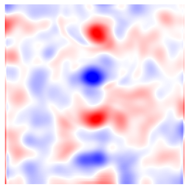
# all_vorticity_fields.dump("../resources/vorticity_fields.npy")
# all_reynolds_numbers.dump("../resources/reynolds_numbers.npy")

# np.savez_compressed("../resources/vorticity_fields.npz", vorticity_fields=all_vorticity_fields)
# np.savez_compressed("../resources/reynolds_numbers.npz", reynolds_numbers=all_reynolds_numbers)
Flattening
Our images have resolution 127x127, so we have 16129 features per frame. We will use a dataset of 1000 frames, and we will need to flatten each frame into a vector of length 16129.
## Convert into a machine-learning dataset by flattening features

# Flatten the vorticity field data
X = np.reshape(all_vorticity_fields, (all_vorticity_fields.shape[0], -1))
# Standardize the data
X = (X - np.mean(X, axis=0)) / np.std(X, axis=0)
y = all_reynolds_numbers

print("Training data has shape: {}".format(X.shape))
print("Training labels have shape: {}".format(y.shape))
Training data has shape: (2000, 16129)
Training labels have shape: (2000,)
How hard is this problem?
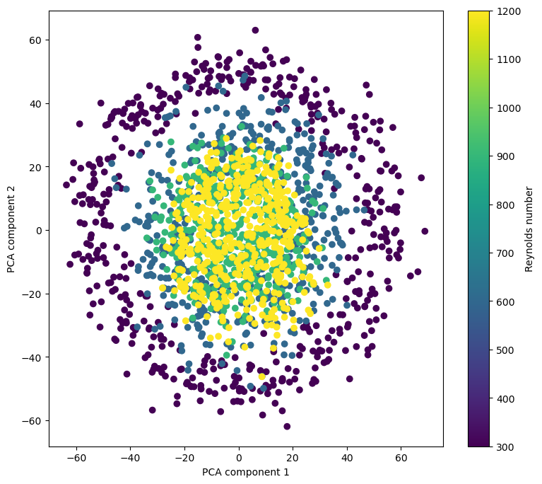
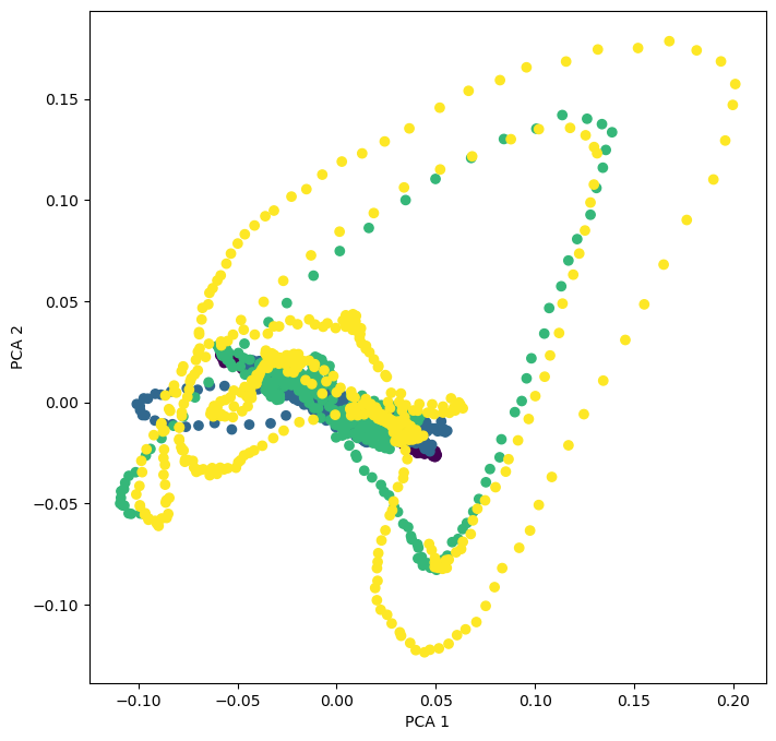
We can try playing with unsupervised embeddings to evaluate the difficulty. Unsupervised techniques can tell us how hard the problem is, and what kind of structure the data has.
Question: Why are these lines?
from sklearn.decomposition import PCA

pca = PCA(n_components=2)
X_pca = pca.fit_transform(X)

plt.figure(figsize=(9, 8))
plt.scatter(X_pca[:, 0], X_pca[:, 1], c=all_reynolds_numbers)
plt.xlabel("PCA component 1")
plt.ylabel("PCA component 2")
plt.colorbar(label="Reynolds number")
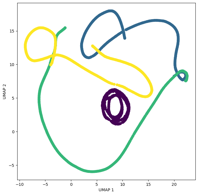
We can also try to visualize the data using a nonlinear embedding technique like UMAP. This method generally does not preserve distances (isometry), but the nearest neighbors of a point in the full 16,000 dimensional space will be preserved in the 2D embedding.
import umap

# Reduce the dimensionality of the data using UMAP
reducer = umap.UMAP(random_state=0)
X_umap = reducer.fit_transform(X)

# Plot the UMAP embedding
plt.figure(figsize=(8, 8))
plt.scatter(X_umap[:, 0], X_umap[:, 1], c=all_reynolds_numbers)
plt.xlabel("UMAP component 1")
plt.ylabel("UMAP component 2")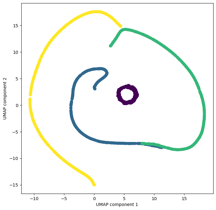
Can we use our domain knowledge to better separate the data?
Inductive biases are when we use our problem knowledge to reduce the number of possible learning models
Like the bias-variance tradeoff, inductive biases allow us to use domain knowledge to “guide” a model, at the expense of flexibility for different problems
For the fluid flow problem, we know that the Navier-Stokes equations contain terms that are quadratic in the velocity field, as well as gradients of the velocity field
We will first try using finite time differences to featurize the data, followed by spatial fourier transforms, which implicitly give information about spatial gradients
# Try finite differences
fd1 = np.gradient(all_vorticity_fields, axis=1).reshape((all_vorticity_fields.shape[0], -1))
fd2 = np.gradient(all_vorticity_fields, axis=2).reshape((all_vorticity_fields.shape[0], -1))
X_fd = np.hstack((fd1, fd2))
X_fd = np.reshape(X_fd, (X_fd.shape[0], -1))
## Augment the feature space with finite differences
X_aug = np.concatenate([X, X_fd], axis=1)
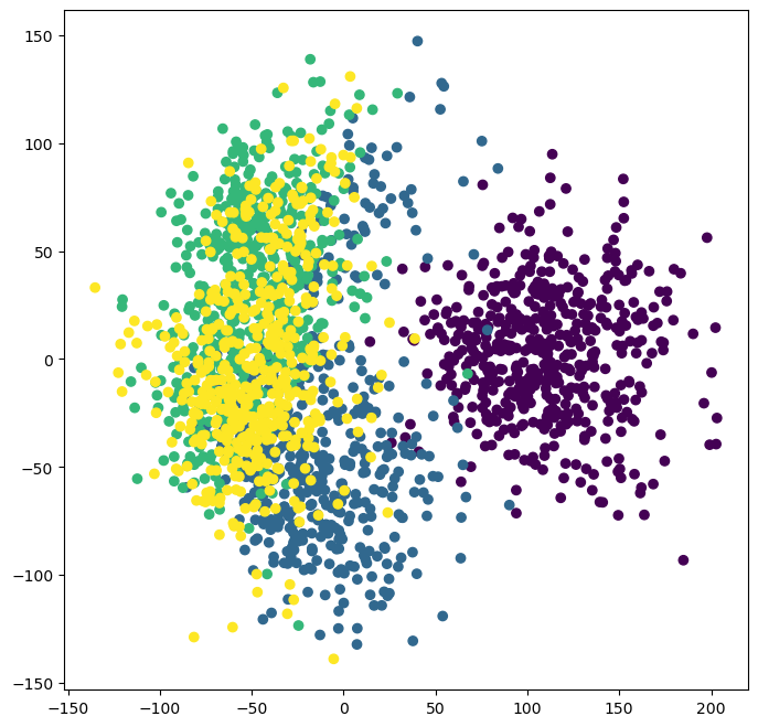
# Try PCA and UMAP on the Fourier coefficients
# Reduce the dimensionality of the data using UMAP
reducer = PCA(n_components=2)
X_pca = reducer.fit_transform(X_fd)
plt.figure(figsize=(8, 8))
plt.scatter(X_pca[:, 0], X_pca[:, 1], c=all_reynolds_numbers)
plt.xlabel("PCA 1")
plt.ylabel("PCA 2")
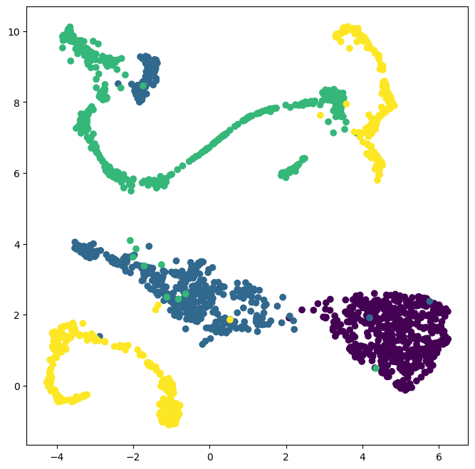
reducer = umap.UMAP(random_state=0)
X_umap = reducer.fit_transform(X_fd)
plt.figure(figsize=(8, 8))
plt.scatter(X_umap[:, 0], X_umap[:, 1], c=all_reynolds_numbers)
plt.xlabel("UMAP 1")
plt.ylabel("UMAP 2")
## Try featurizing with 2D Fourier coefficients

# Calculate the 2D Fourier coefficients
X_fft = np.fft.fft2(all_vorticity_fields)

# Convert to power spectrum
X_fft = np.reshape(np.abs(X_fft)**2, (X_fft.shape[0], -1))

# Try PCA and UMAP on the Fourier coefficients

# Reduce the dimensionality of the data using UMAP
reducer = PCA(n_components=2)
X_pca = reducer.fit_transform(X_fft)
plt.figure(figsize=(8, 8))
plt.scatter(X_pca[:, 0], X_pca[:, 1], c=all_reynolds_numbers)


reducer = umap.UMAP(random_state=0)
X_umap = reducer.fit_transform(X_fft)
plt.figure(figsize=(8, 8))
plt.scatter(X_umap[:, 0], X_umap[:, 1], c=all_reynolds_numbers)
Let’s try training a model to predict Reynolds number
As a baseline, we’ll use multinomial logistic regression, which extends logistic regression to more than two classes
Generally, we prefer using a simple model as a baseline, before moving to more complex models
In the machine learning literature, baselines and ablations are important for establishing the value of a new model or architecture
from sklearn.linear_model import LogisticRegression
from sklearn.model_selection import train_test_split
from sklearn.metrics import confusion_matrix

## Shuffle the data and split into training and test sets
sel_inds = np.random.permutation(X.shape[0])[:400]
X_all, y_all = X[sel_inds], y[sel_inds]
X_train, X_test, y_train, y_test = train_test_split(X_all, y_all, test_size=0.4, random_state=0)
# X_train, X_test, y_train, y_test = train_test_split(X, y, test_size=0.4, random_state=0)


model_logistic = LogisticRegression()
model_logistic.fit(X_train, y_train)
y_pred_logistic = model_logistic.predict(X_test)

print("Training set score: {:.2f}".format(model_logistic.score(X_train, y_train)))
print("Test set score: {:.2f}".format(model_logistic.score(X_test, y_test)))

plt.imshow(confusion_matrix(y_test, y_pred_logistic))
plt.xlabel("Predicted")
plt.ylabel("True")
plt.xticks(np.arange(len(re_vals)), re_vals);
plt.yticks(np.arange(len(re_vals)), re_vals);
Training set score: 1.00
Test set score: 0.63
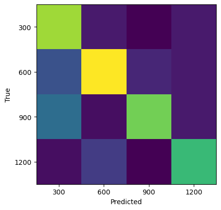
from sklearn.neural_network import MLPClassifier
from sklearn.model_selection import train_test_split
from sklearn.metrics import confusion_matrix

X_train, X_test, y_train, y_test = train_test_split(X, y, test_size=0.4, random_state=0)

# A 4 layer neural network with 10 hidden units in each layer
mlp = MLPClassifier(hidden_layer_sizes=(3, 3), random_state=0)
mlp.fit(X_train, y_train)
y_pred = mlp.predict(X_test)

print("Training set score: {:.2f}".format(mlp.score(X_train, y_train)))
print("Test set score: {:.2f}".format(mlp.score(X_test, y_test)))

plt.imshow(confusion_matrix(y_test, y_pred))
plt.xlabel("Predicted")
plt.ylabel("True")
plt.xticks(np.arange(len(re_vals)), re_vals);
plt.yticks(np.arange(len(re_vals)), re_vals);
Training set score: 0.89
Test set score: 0.76
Training set score: 0.89
Test set score: 0.76
Can we do better? How deep should we go?
Model choices = hyperparameter tuning. Recall that any “choice” that affects model complexity is a hyperparameter, including the choice of model itself, the optimizer, the learning rate, the number of layers, the number of neurons per layer, the activation function, etc. Here, we will focus on the number and width of layers
We use cross-validation (we split train into validation sets)
To search over hyperparameters, we use scikit-learn’s
GridSearchCV, which uses the same API as a standard model, but which internally trains and evaluates the model on all possible hyperparameter combinations with cross-validation
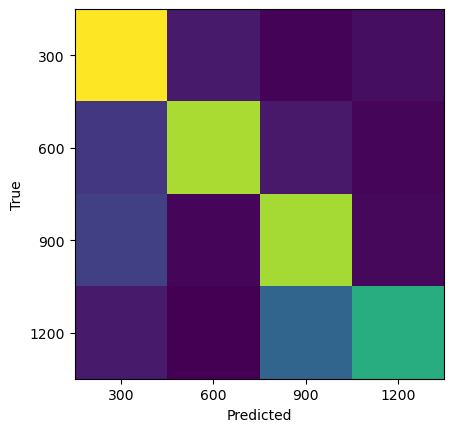
## Tuning hyperparameters with sklearn built-in grid search and cross-validation
from sklearn.model_selection import GridSearchCV
param_grid = {'hidden_layer_sizes': [(3, 3, 3), (5, 5), (7, 5, 3)]}
grid = GridSearchCV(MLPClassifier(), param_grid, cv=5)
grid.fit(X_train, y_train)
print("Best cross-validation score: {:.2f}".format(grid.best_score_))
print("Best parameters: ", grid.best_params_)
print("Train set score: {:.2f}".format(grid.score(X_train, y_train)))
print("Test set score: {:.2f}".format(grid.score(X_test, y_test)))
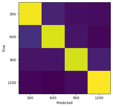
plt.imshow(confusion_matrix(y_test, grid.predict(X_test)))
plt.xlabel("Predicted")
plt.ylabel("True")
plt.xticks(np.arange(len(re_vals)), re_vals);
plt.yticks(np.arange(len(re_vals)), re_vals);Best cross-validation score: 0.80
Best parameters: {'hidden_layer_sizes': (7, 5, 3)}
Train set score: 0.99
Test set score: 0.89
Best cross-validation score: 0.79
Best parameters:  {'hidden_layer_sizes': (5, 5)}
Test set score: 0.83
## Use the best hyperparameters
mlp = MLPClassifier(**grid.best_params_, random_state=0)
mlp.fit(X_train, y_train)
y_pred_train = mlp.predict(X_train)
y_pred_test = mlp.predict(X_test)

print("Training set score: {:.2f}".format(mlp.score(X_train, y_train)))
print("Test set score: {:.2f}".format(mlp.score(X_test, y_test)))

plt.imshow(confusion_matrix(y_test, y_pred))
plt.xlabel("Predicted")
plt.ylabel("True")
plt.xticks(np.arange(len(re_vals)), re_vals);
plt.yticks(np.arange(len(re_vals)), re_vals);
Training set score: 0.97
Test set score: 0.85
Visualize the decision boundary
Our images live in a high-dimensional feature space, but we can still visualize the decision boundary in a lower-dimensional space using the embedding techniques we learned about last week
We will visualize our decision boundary in this embedding space
# Train embedding on the data
reducer = umap.UMAP(random_state=0)
reducer.fit(X)
X_umap_train = reducer.transform(X_train)
X_umap_test = reducer.transform(X_test)
plt.figure(figsize=(8, 8))
plt.scatter(X_umap_train[:, 0], X_umap_train[:, 1], c=y_train)
plt.scatter(X_umap_test[:, 0], X_umap_test[:, 1], c=y_test, marker='o')
plt.xlabel("UMAP 1")
plt.ylabel("UMAP 2")
plt.title("Ground Truth")
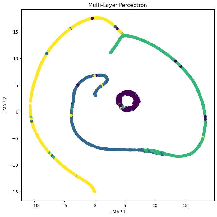
plt.figure(figsize=(8, 8))
plt.scatter(X_umap_train[:, 0], X_umap_train[:, 1], c=y_pred_train)
plt.scatter(X_umap_test[:, 0], X_umap_test[:, 1], c=y_pred_test, marker='o')
plt.xlabel("UMAP 1")
plt.ylabel("UMAP 2")
plt.title("Multi-Layer Perceptron")
plt.figure(figsize=(8, 8))
# plt.scatter(X_umap_train[:, 0], X_umap_train[:, 1], c=y_train)
# plt.scatter(X_umap_test[:, 0], X_umap_test[:, 1], c=y_pred_logistic, marker='o')
# plt.xlabel("UMAP 1")
# plt.ylabel("UMAP 2")
# plt.title("Logistic Regression")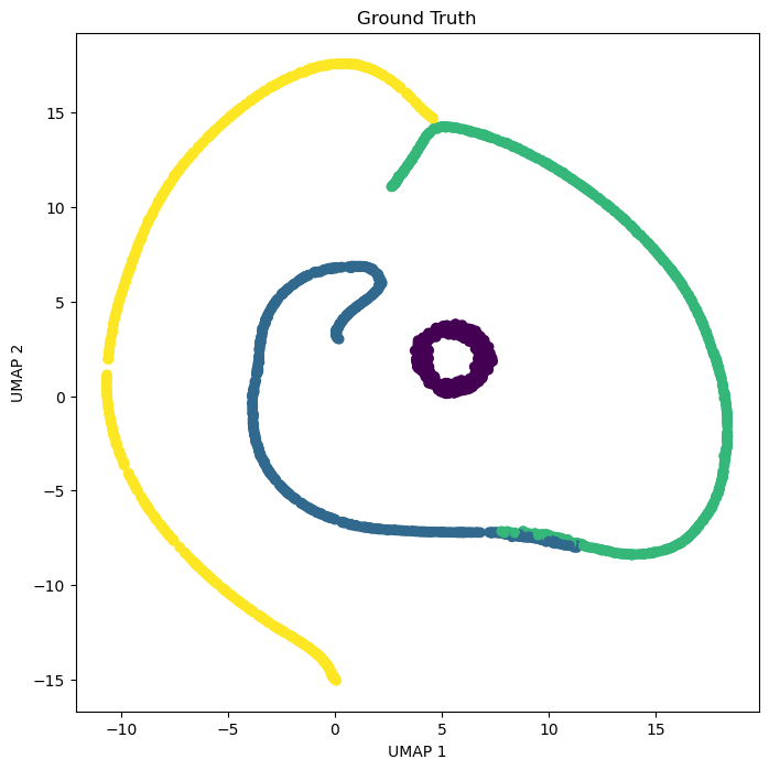
<Figure size 800x800 with 0 Axes>How big is our model?
Our final neural network maps from features to 4 classes, with 1 hidden layers containing 10 neurons. This means we have around 160,000 trainable parameters
grid.best_params_{'hidden_layer_sizes': (7,)}A convolutional neural network
Can we process the images in a more parameter-efficient way?
The Multi-Layer oerceptron model we used above has a lot of trainable parameters, since it maps flattened images that have features into a single output. Even a linear model would have 16129 parameters!
We know that turbulent flows have a lot of spatial structure, and that the Navier-Stokes equations are local in space. Can we build this property into our model?
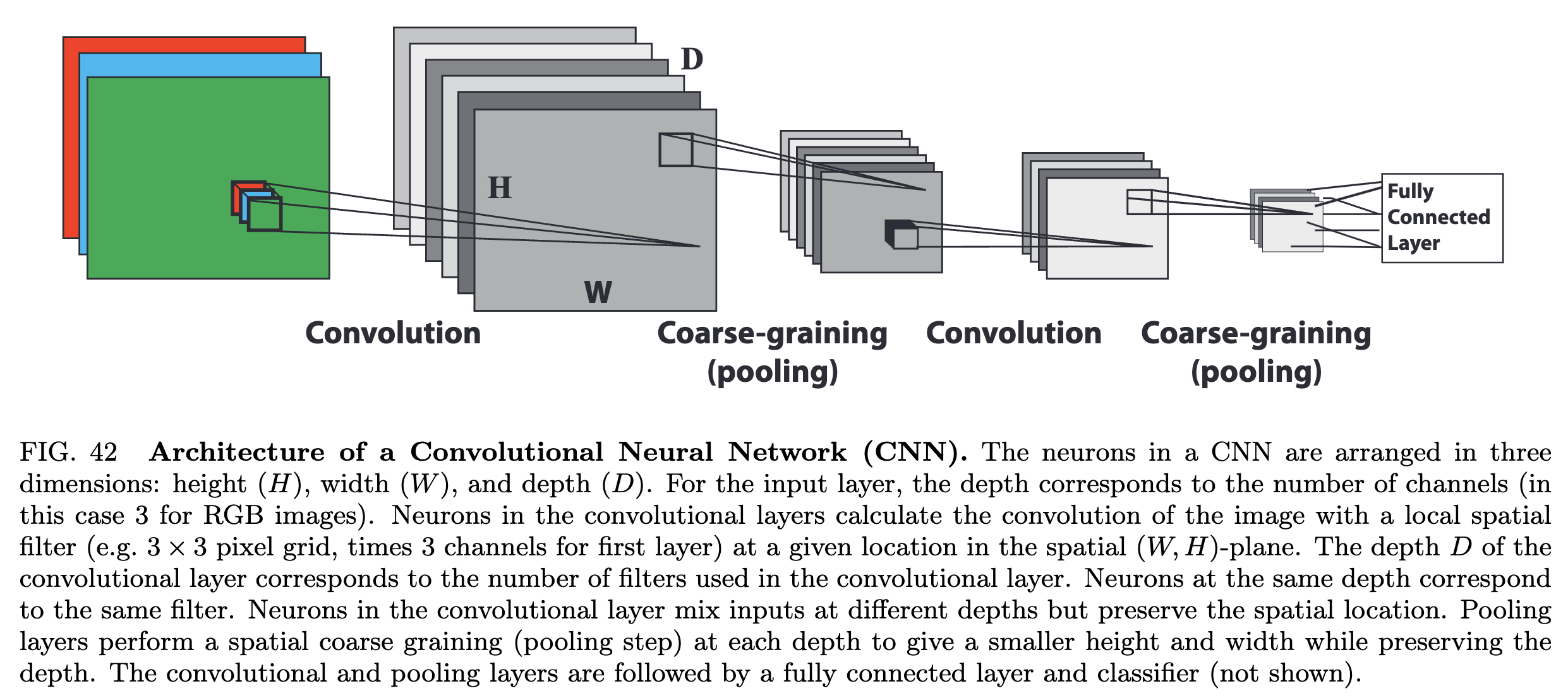
Image from Mehta et al. 2018
In a convolutional neural network (CNN), we avoid explicitly flattening the image, and instead apply a series of trainable convolutional filters to the image
Recall that convolutional filters are usually small kernels, like or images, that we slide across the image. The output of a discrete convolution is a new image, where each pixel is a combination of pixel neighborhoods from the previous image
Our image classifier needs to map from an image to a single output, and so CNN also includes a series of pooling layers, which downsample the intermediate images
After the image becomes sufficiently small, we then flatten it and apply a standard fully-connected neural network to the flattened image
As a starting point, we will leave our input dataset in the form of images. So instead of our training data having the shape , it will have the shape
## Convert into a machine-learning dataset by flattening features
X = np.copy(all_vorticity_fields)[..., None]
# Standardize the data
X = (X - np.mean(X, axis=0)) / np.std(X, axis=0)
y = np.unique(all_reynolds_numbers, return_inverse=True)[1] # Convert labels to integers
from sklearn.model_selection import train_test_split
from sklearn.metrics import confusion_matrix
X_train, X_test, y_train, y_test = train_test_split(X, y, test_size=0.4, random_state=0)
print("Training data has shape: {}".format(X_train.shape))
print("Training labels have shape: {}".format(y_train.shape))
print("Test data has shape: {}".format(X_test.shape))
print("Test labels have shape: {}".format(y_test.shape))
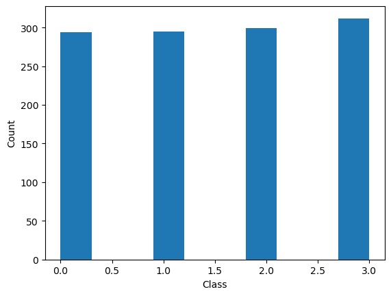
plt.hist(y_train)
plt.xlabel("Class")
plt.ylabel("Count")Training data has shape: (1200, 127, 127, 1)
Training labels have shape: (1200,)
Test data has shape: (800, 127, 127, 1)
Test labels have shape: (800,)
Training data has shape: (1200, 127, 127, 1)
Training labels have shape: (1200,)
Test data has shape: (800, 127, 127, 1)
Test labels have shape: (800,)
Implementing a CNN
Technical setup: We implement our CNN using JAX, a library for automatic differentiation and GPU acceleration. PyTorch is an alternative library with similar features. We thus need to install JAX and its optimization library, optax. We will now implement a CNN using JAX, a library for automatic differentiation and GPU acceleration. PyTorch is an alternative library with similar features. We thus need to install JAX and its optimization library, optax.
pip install jax jaxlib optaxOur implementation will inherit the fit/predict API structure used for objects in scikit-learn.
Problem formulation: Because our dataset describes a classification (categorical) problem, our model will return a final layer of size 4. The continuous values in this vector are the logits of the model. In the last step, the four numbers are converted into probability scores for each of the four classes using the softmax function
During training, these values are then used to compute the cross-entropy loss, which is a measure of how well the model is doing at predicting the correct class
where is the true label of training data point and is the predicted label.
During prediction, the model will use a “hard max” (argmax) to convert the softmax probabilities into a single class prediction
where is the predicted probability of class for data point .
import jax
import jax.numpy as jnp
from jax import grad, jit, random, value_and_grad
import optax # An optimization library for JAX
from sklearn.base import BaseEstimator, ClassifierMixin

class CNNClassifier(BaseEstimator, ClassifierMixin):
    """
    A Convolutional Neural Network (CNN) classifier implemented using JAX and NumPy.

    Parameters:
        learning_rate (float): The learning rate for the optimizer
        epochs (int): The number of training epochs
        batch_size (int): The batch size for training
        random_state (int): The random seed for reproducibility


    """
    def __init__(self, learning_rate=0.001, epochs=10, batch_size=32, random_state=0, store_history=True):

        ## Set hyperparameters
        self.learning_rate = learning_rate
        self.epochs = epochs
        self.batch_size = batch_size

        ## Set trainable internal parameters and object state
        self.params = None
        self.opt_state = None

        self.random_state = random_state
        # JAX uses PRNG objects to control random number generation
        self.rng = random.PRNGKey(random_state)

        self.store_history = store_history
        if self.store_history:
            self.loss_history = []


    def _init_params(self, input_shape, num_classes):
        """
        Initialize the trainable model parameters

        Args:
            input_shape (tuple): The shape of the input data
            num_classes (int): The number of classes in the classification task

        Returns:
            None

        """
        self.params = {
            "conv1": {
                "w": random.normal(self.rng, (3, 3, input_shape[-1], 32)),
                "b": jnp.zeros((32,))
            },
            "fc": {
                "w": random.normal(self.rng, (32 * (input_shape[0] // 2) * (input_shape[1] // 2), num_classes)),
                "b": jnp.zeros((num_classes,))
            }
        }

    def _forward(self, params, X):
        """
        Forward pass of the CNN model. Given a batch of data, compute the logits
        corresponding to each class.

        Args:
            params (dict): Dictionary containing the model parameters
            X (numpy.ndarray): Batch of input data

        Returns:
            numpy.ndarray: Logits for each class
        """
        def relu(x):
            return jnp.maximum(0, x)

        # Convolution layer transforms the input image from a shape of
        # (batch_size, height, width, channels), here (64, 128, 128, 1), to a shape of
        # (batch_size, height, width, num_filters), here (64, 128, 128, 32)
        conv1_out = jax.lax.conv_general_dilated(
            X,
            params["conv1"]["w"],
            window_strides=(1, 1),
            dimension_numbers=("NHWC", "HWIO", "NHWC"),
            padding="SAME"
        )
        conv1_out = relu(conv1_out + params["conv1"]["b"])

        # Pooling layer shrinks the intermediate representation to
        # (batch_size, height // 2, width // 2, num_filters), here (64, 64, 64, 32)
        pool_out = jax.lax.reduce_window(
            conv1_out,
            0.0,
            jax.lax.add,
            window_dimensions=(1, 2, 2, 1),
            window_strides=(1, 2, 2, 1),
            padding="VALID"
        )

        # The flattening operation reshapes the tensor to (batch_size, num_features),
        # here (64, 64 * 64 * 32), and then computes the logits
        flattened = pool_out.reshape((X.shape[0], -1))
        logits = jnp.dot(flattened, params["fc"]["w"]) + params["fc"]["b"]

        return logits

    def _loss(self, params, X, y):
        """
        Compute the cross-entropy loss between the model predictions and the true labels

        The cross-entropy loss is defined as:

        L = -1/N * sum_i sum_j y_ij * log(p_ij)

        where N is the number of samples, y_ij is 1 if sample i belongs to class j, and p_ij
        is the predicted probability that sample i belongs to class j.

        Args:
            params (dict): Dictionary containing the model parameters
            X (numpy.ndarray): Batch of input data
            y (numpy.ndarray): Batch of labels

        Returns:
            numpy.ndarray: The cross-entropy loss, averaged over the batch
        """
        logits = self._forward(params, X) # Returns the logits for each class
        y_onehot = jax.nn.one_hot(y, logits.shape[-1])
        loss = -jnp.mean(jnp.sum(y_onehot * jax.nn.log_softmax(logits), axis=-1))
        return loss

    def _update(self, params, opt_state, X, y):
        """
        Compute the gradients of the loss with respect to the model parameters and
        update the model

        Args:
            params (dict): Dictionary containing the model parameters
            opt_state (dict): Dictionary containing the optimizer state
            X (numpy.ndarray): Batch of input data
            y (numpy.ndarray): Batch of labels

        Returns:
            dict: Updated model parameters
            dict: Updated optimizer state
            float: The loss value
        """
        loss, grads = value_and_grad(self._loss)(params, X, y)
        updates, opt_state = self.optimizer.update(grads, opt_state, params)
        params = optax.apply_updates(params, updates)
        return params, opt_state, loss

    def fit(self, X, y):
        """
        Fit the CNN model to the training data

        Args:
            X (numpy.ndarray): Training data of shape (num_samples, height, width, channels)
            y (numpy.ndarray): Training labels of shape (num_samples,)
        """

        ## Initialize the model parameters and optimizer at the first call to fit
        if self.params is None:
            input_shape = X.shape[1:]
            num_classes = len(jnp.unique(y))
            self._init_params(input_shape, num_classes)
            self.optimizer = optax.adam(self.learning_rate)
            self.opt_state = self.optimizer.init(self.params)

        ## Optimization loop
        for epoch in range(self.epochs):
            perm = random.permutation(self.rng, X.shape[0])
            X, y = X[perm], y[perm]

            ## iterate over the dataset in mini-batches
            for i in range(0, X.shape[0], self.batch_size):
                X_batch = X[i:i + self.batch_size]
                y_batch = y[i:i + self.batch_size]
                self.params, self.opt_state, loss = self._update(self.params, self.opt_state, X_batch, y_batch)

            if self.store_history:
                self.loss_history.append(loss)
                print(f"Epoch {epoch + 1}/{self.epochs}, Loss: {loss:.4f}")

    def predict(self, X):
        """
        Make predictions on new data

        Args:
            X (numpy.ndarray): New data of shape (num_samples, height, width, channels)

        Returns:
            numpy.ndarray: Predicted labels
        """
        logits = self._forward(self.params, X)
        return jnp.argmax(logits, axis=-1)
## Fit the CNN model
# # Train and predict
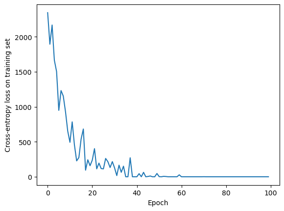
model = CNNClassifier(learning_rate=0.0001, epochs=100, batch_size=16)
model.fit(X_train, y_train)
plt.plot(model.loss_history)
plt.xlabel("Epoch")
plt.ylabel("Cross-entropy loss on training set")
Epoch 1/100, Loss: 2344.1562
Epoch 2/100, Loss: 1893.5312
Epoch 3/100, Loss: 2167.5793
Epoch 4/100, Loss: 1665.8159
Epoch 5/100, Loss: 1502.6653
Epoch 6/100, Loss: 948.9930
Epoch 7/100, Loss: 1231.2178
Epoch 8/100, Loss: 1153.6851
Epoch 9/100, Loss: 929.2589
Epoch 10/100, Loss: 652.1995
Epoch 11/100, Loss: 492.6980
Epoch 12/100, Loss: 784.1656
Epoch 13/100, Loss: 455.9197
Epoch 14/100, Loss: 227.0690
Epoch 15/100, Loss: 274.9376
Epoch 16/100, Loss: 538.9522
Epoch 17/100, Loss: 682.2462
Epoch 18/100, Loss: 94.5268
Epoch 19/100, Loss: 242.6960
Epoch 20/100, Loss: 158.2983
Epoch 21/100, Loss: 236.4017
Epoch 22/100, Loss: 401.7467
Epoch 23/100, Loss: 113.3213
Epoch 24/100, Loss: 195.1394
Epoch 25/100, Loss: 117.2153
Epoch 26/100, Loss: 113.0649
Epoch 27/100, Loss: 261.6731
Epoch 28/100, Loss: 215.6727
Epoch 29/100, Loss: 132.2099
Epoch 30/100, Loss: 216.4857
Epoch 31/100, Loss: 127.0312
Epoch 32/100, Loss: 17.0016
Epoch 33/100, Loss: 165.9627
Epoch 34/100, Loss: 63.9287
Epoch 35/100, Loss: 151.2602
Epoch 36/100, Loss: -0.0000
Epoch 37/100, Loss: -0.0000
Epoch 38/100, Loss: 271.1634
Epoch 39/100, Loss: -0.0000
Epoch 40/100, Loss: -0.0000
Epoch 41/100, Loss: -0.0000
Epoch 42/100, Loss: 44.3639
Epoch 43/100, Loss: 0.5360
Epoch 44/100, Loss: 63.3394
Epoch 45/100, Loss: -0.0000
Epoch 46/100, Loss: 4.4885
Epoch 47/100, Loss: 11.2855
Epoch 48/100, Loss: -0.0000
Epoch 49/100, Loss: -0.0000
Epoch 50/100, Loss: 46.8023
Epoch 51/100, Loss: 2.0290
Epoch 52/100, Loss: -0.0000
Epoch 53/100, Loss: 6.1905
Epoch 54/100, Loss: 4.0004
Epoch 55/100, Loss: -0.0000
Epoch 56/100, Loss: -0.0000
Epoch 57/100, Loss: -0.0000
Epoch 58/100, Loss: -0.0000
Epoch 59/100, Loss: -0.0000
Epoch 60/100, Loss: 27.7790
Epoch 61/100, Loss: -0.0000
Epoch 62/100, Loss: -0.0000
Epoch 63/100, Loss: -0.0000
Epoch 64/100, Loss: -0.0000
Epoch 65/100, Loss: -0.0000
Epoch 66/100, Loss: -0.0000
Epoch 67/100, Loss: -0.0000
Epoch 68/100, Loss: 0.0001
Epoch 69/100, Loss: -0.0000
Epoch 70/100, Loss: -0.0000
Epoch 71/100, Loss: 0.8741
Epoch 72/100, Loss: -0.0000
Epoch 73/100, Loss: -0.0000
Epoch 74/100, Loss: -0.0000
Epoch 75/100, Loss: -0.0000
Epoch 76/100, Loss: -0.0000
Epoch 77/100, Loss: -0.0000
Epoch 78/100, Loss: -0.0000
Epoch 79/100, Loss: -0.0000
Epoch 80/100, Loss: -0.0000
Epoch 81/100, Loss: -0.0000
Epoch 82/100, Loss: -0.0000
Epoch 83/100, Loss: -0.0000
Epoch 84/100, Loss: -0.0000
Epoch 85/100, Loss: -0.0000
Epoch 86/100, Loss: -0.0000
Epoch 87/100, Loss: -0.0000
Epoch 88/100, Loss: -0.0000
Epoch 89/100, Loss: -0.0000
Epoch 90/100, Loss: -0.0000
Epoch 91/100, Loss: -0.0000
Epoch 92/100, Loss: -0.0000
Epoch 93/100, Loss: -0.0000
Epoch 94/100, Loss: -0.0000
Epoch 95/100, Loss: -0.0000
Epoch 96/100, Loss: -0.0000
Epoch 97/100, Loss: -0.0000
Epoch 98/100, Loss: -0.0000
Epoch 99/100, Loss: -0.0000
Epoch 100/100, Loss: -0.0000
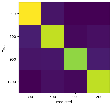
y_pred_train = model.predict(X_train)
y_pred_test = model.predict(X_test)
print("Training set score: {:.2f}".format(np.mean(y_pred_train == y_train)))
print("Test set score: {:.2f}".format(np.mean(y_pred_test == y_test)))
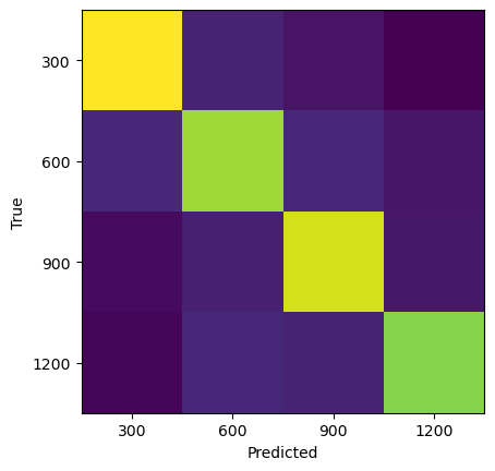
plt.imshow(confusion_matrix(y_test, y_pred_test))
plt.xlabel("Predicted")
plt.ylabel("True")
plt.xticks(np.arange(len(re_vals)), re_vals);
plt.yticks(np.arange(len(re_vals)), re_vals);
Training set score: 1.00
Test set score: 0.78
How many parameters did that take?
The convolutional layer has parameters. In our case, , ,
The fully connected layer has parameters. In our case,
The total number of parameters is therefore
conv_shape = model.params['conv1']['w'].shape
fc_shape = model.params['fc']['w'].shape

print(f"The convolutional layer has shape {conv_shape} with {np.prod(conv_shape)} parameters")
print(f"The fully connected layer has shape {fc_shape} with {np.prod(fc_shape)} parameters")
The convolutional layer has shape (3, 3, 1, 32) with 288 parameters
The fully connected layer has shape (127008, 4) with 508032 parameters
Inductive biases in machine learning
By using a CNN, we managed to get both higher accuracy and use a lower number of trainable parameters than the MLP. The key reason for this is that the CNN architecture has an inductive bias for datasets with spatial translation invariance: the same convolutional filter can be applied to different parts of the image, and so the model doesn’t need to learn a different filter for each part of the image. Generally, the success of CNNs in computer vision is due to this inductive bias for spatial translation invariance, which happens to describe many types of image data that are common in nature.
However, there is no free lunch: the CNN architecture performs poorly on datasets that do not have spatial translation invariance. For example, CNN tend to perform poorly on image datasets that require absolute spatial position information, such as images of puzzles or graphs. Likewise, CNNs are not suited for data in which there is no metric by which to define a “local” region, such as tabular datasets.
This CNN represents a vignette of a common trade-off in scientific machine learning: we can use our domain knowledge to guide our model choices, and to get better performance with fewer parameters. But this comes at the expense of flexibility for other datasets. This introduces the question of when we should encode our domain knowledge, versus leaving the model to discover it (potentially at the expense of performance or additional training time). The “bitter lesson” often invoked in modern machine learning argues that, as the speed of computers and available data increases, the amount of domain-specific knowledge we should encode should decrease.
mlp.fit(X_train, y_train)
y_pred_train = mlp.predict(X_train)
y_pred_test = mlp.predict(X_test)

print("Training set score: {:.2f}".format(mlp.score(X_train, y_train)))
print("Test set score: {:.2f}".format(mlp.score(X_test, y_test)))