Preamble: Run the cells below to import the necessary Python packages
This notebook created by William Gilpin. Consult the course website for all content and GitHub repository for raw files and runnable online code.

import numpy as np
import matplotlib.pyplot as plt
%matplotlib inline

## Import plot settings
import requests
code = requests.get("https://raw.githubusercontent.com/williamgilpin/cphy/main/cphy/template.py", timeout=10).text
exec(code, globals(), globals())

## Initialize code for plotting spheres
from matplotlib.collections import EllipseCollection
def make_ellipses(coords, r, ax=None):
    """Given a set of coordinates, return an EllipseCollection object that can be used
    to plot disks of radius r at each of the given coordinates."""
    if ax is None:
        ax = plt.gca()
    w0 = np.full(len(coords), 2*r)
    h0 = np.full(len(coords), 2*r)
    ec = EllipseCollection(
        w0, h0, np.zeros(len(coords)),
        units='xy',                      # widths/heights are in data units
        offsets=coords, offset_transform=ax.transData,
        facecolor='b', edgecolor='none', alpha=0.6
    )
    return ec
Gradient-free optimization
We saw before that many optimization methods implicitly require the locally-computed gradient of the potential , either computed explicitly or using a heuristic like finite-difference approximation or automatic differentiation.
For problems for which the gradient is impossible to compute (i.e. discrete systems like cellular automata), we can genetic algorithms to optimize systems. But what about problems where it is possible to physically perform small perturbations, in the sense of applying changes that lead to bounded changes in the potential. We can’t necessarily fully differentiate such systems, because the energy function itself is discontinuous in the perturbation. An example of this case is the Ising model Hamiltonian,
where . When the number of spins is large (), the change in energy due to flipping a single spin , is bounded. However, because the optimization variables are discrete, we cannot directly take the gradient of this function.
In other cases, the gradient exists and we could try directly approximating it using finite differences. However, this fails in high dimensions because approximating a -dimensional gradient by finite differences costs evaluations of the potential, where is the dimensionality of the system. If the potential is expensive to evaluate, this can be prohibitive.
Monte Carlo methods can be used to optimize a potential without computing its gradient. This can be useful either when the gradient does not exist, or it is very expensive to compute. Like gradient methods, they exploit small perturbations to find local information about the potential to guide the search.
The Metropolis algorithm
Given a system I want to optimize, suppose that I have a scalar energy function that depends on a vector of variables that describe the system’s configuration.
We initialize a system in a given configuration,
We apply a perturbation to the system’s parameters, resulting in a new configuration . Ideally, we have a method of perturbing the system such that the resulting change in the energy is bounded, even if it’s not continuous.
We compute the change in energy between the proposed (perturbed) and original configuration,
If , we immediately accept the update,
If , we accept the new configuration with probability , where is the inverse temperature of the sampling process.
Properties of the Metropolis algorithm.
The inverse temperature as a critical hyperparameter that controls properties of the optimization. When , then we never accept higher energy steps. This corresponds to greedy dynamics, in which the system can only descend in energy. This is the abstract equivalent of the overdamped dynamics we saw in gradient descent. Conversely, when , then we always accept the update, and so the optimization decouples from the energy of the state.
In both extremes, the decision whether to accept a step becomes fully deterministic. In practice, Monte Carlo methods work best when they are maximally stochastic, and so, in practice, is usually chosen so that we accept roughly half of all proposed updates.
Why not always set large?. We might think that the fastest convergence would occur if we always accepted updates that lower the energy, and always rejected updates that increase the energy (equivalent to ). The probabilistic update rule here represents a way for the optimizer to avoid getting stuck in local minima.
Implementing the Metropolis optimizer
To implement the random choice, We will draw a random number, , from a uniform distribution between 0 and 1. If , we accept a higher-energy configuration. Otherwise, we reject the new configuration and keep the old one. We will vectorize our implementation, in order to allow us to optimize particles starting at multiple initial positions simultaneously.
class MetropolisMonteCarlo:
    """
    Metropolis algorithm for optimizing a loss function.

    Attributes:
        energy (function): The loss function to be minimized
        beta (float): The inverse temperature
        amplitude (float): The amplitude of the perturbation applied to the state
        max_iter (int): The maximum number of iterations
        random_state (int): The random seed
        store_history (bool): Whether to store the history of the state
    """
    def __init__(
            self,
            loss,
            beta=1.0,
            amplitude=1.0,
            max_iter=500,
            random_state=None,
            store_history=False
        ):
        self.energy = loss
        self.beta = beta
        self.amplitude = amplitude
        self.n_iter = max_iter
        self.store_history = store_history
        self.random_state = random_state

        self.store_history = store_history
        if self.store_history:
            self.Xs = []
            self.losses = []

    def perturb(self, X):
        """
        Randomly the state of the system.

        Args:
            X (ndarray): The current state of the system

        Returns:
            Xp (ndarray): The perturbed state of the system
        """
        Xp = X + self.amplitude * np.random.normal(size=X.shape)
        return Xp

    def update(self, X):
        """
        Update the state of the system.

        Args:
            X (ndarray): The current state of the system

        Returns
            X (ndarray): The updated state of the system
        """

        Xp = self.perturb(X)
        e_delta = self.energy(Xp) - self.energy(X)

        # Create vector of update or not
        rho = np.random.random(X.shape[0])
        do_update = np.zeros(X.shape[0])
        do_update[e_delta < 0] = 1
        do_update[rho < np.exp(-self.beta * e_delta)] = 1

        X_out = X.copy()
        X_out[do_update == 1] = Xp[do_update == 1]
        return X_out

    def fit(self, X):
        """
        Run the Monte Carlo simulation.

        Args:
            X (ndarray): The initial state of the system

        Returns:
            X (ndarray): The final state of the system
        """
        np.random.seed(self.random_state)
        if self.store_history:
            self.Xs.append(X)
            self.losses.append(self.energy(X))
        for _ in range(self.n_iter):
            X = self.update(X)
            if self.store_history:
                self.Xs.append(X)
                self.losses.append(self.energy(X))
        return X
In addition to specifying the value of the inverse temperature hyperparameter , we also need to specify the amplitude of the random perturbation applied to the system. This parameter is analogous to the learning rate in gradient descent.
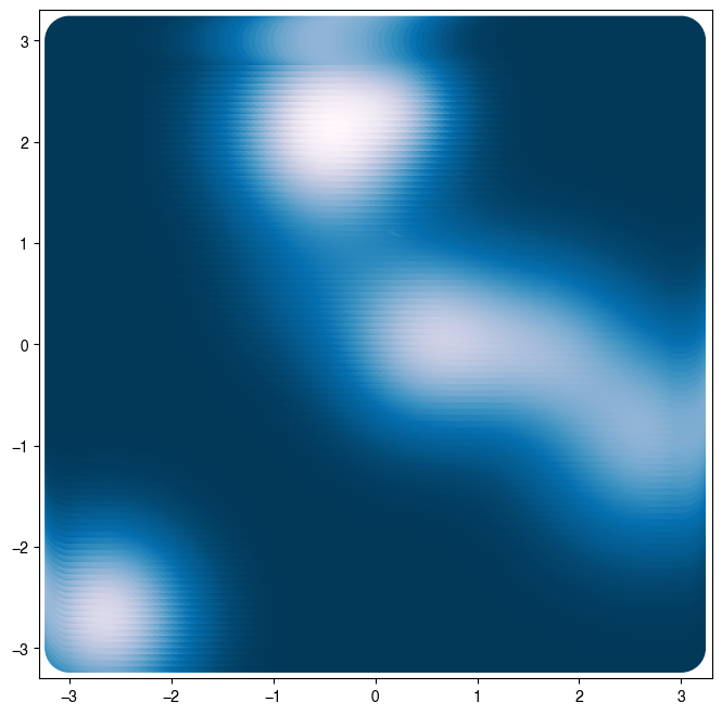
A random two-dimensional loss landscape
To gain some intuition for the behavior of the Metropolis algorithm compared to gradient-descent, we can revisit the two-dimensional random loss landscape. We start by implementing the loss landscape as a standalone object.
class RandomLossLandscape:
    """
    Creates a random two-dimensional loss landscape with multiple circular gaussian wells

    Args:
        d (int): number of dimensions for the loss landscape
        n_wells (int): number of gaussian wells
        random_state (int): random seed

    """

    def __init__(self, d=2, n_wells=3, random_state=None):

        # Fix the random seed
        self.random_state = random_state
        np.random.seed(random_state)

        # Select random well locations, widths, and amplitudes
        self.locs = (2 * np.random.uniform(size=(n_wells, d)) - 1) * 3
        self.widths = np.random.rand(n_wells)[None, :]
        self.coeffs = np.random.random(n_wells)
        self.coeffs /= np.sum(self.coeffs) # normalize the amplitudes

    def _gaussian_well(self, X, width=1):
        """
        A single gaussian well centered at 0 with specified width

        Args:
            X (np.ndarray): points at which to compute the gaussian well. This should
                be of shape (n_batch, n_dim)
            width (float): The width of the gaussian well

        Returns:
            np.ndarray: The value of the gaussian well at points X. The shape of the output
                is (n_batch,)
        """
        return -np.exp(-np.sum((X / width) ** 2, axis=1))

    def _grad_gaussian_well(self, X, width=1):
        return -2 * X / (width ** 2) * self._gaussian_well(X, width)[:, None, :]

    def grad(self, X):
        # Arg shape before summation is (n_batch, n_dim, n_wells)
        return np.sum(
            self.coeffs * self._grad_gaussian_well(X[..., None] - self.locs.T[None, :], self.widths),
            axis=-1
        )

    def loss(self, X):
        """
        Compute the loss landscape at points X

        Args:
            X (np.ndarray): points at which to compute the loss landscape. This should
                be of shape (n_batch, n_dim)
            width (float): The width of the gaussian wells

        Returns:
            np.ndarray: loss landscape at points X

        Notes:
            The loss landscape is computed as the sum of the individual gaussian wells
            The shape of the argument to np.sum is (n_batch, n_wells)
        """
        return np.sum(
            self._gaussian_well(X[..., None] - self.locs.T[None, :], self.widths) * self.coeffs,
            axis=1
        )

    def __call__(self, X):
        return self.loss(X)


# Instantiate a random loss
loss = RandomLossLandscape(random_state=0, n_wells=8)
# loss.plot()
# plt.axis('off')

plt.figure(figsize=(8, 8))

## First we plot the scalar field at high resolution
x = np.linspace(-3, 3, 100)
y = np.linspace(-3, 3, 100)
xx, yy = np.meshgrid(x, y)
X = np.array([xx.ravel(), yy.ravel()]).T
print(X.shape)
Z = loss(X) # same as loss.loss(X) because class is callable
plt.scatter(X[:, 0], X[:, 1], c=Z, s=1000)
(10000, 2)
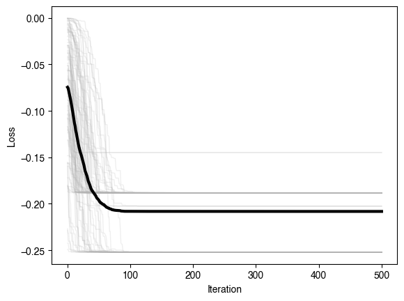
We can now initialize the Metropolis Monte Carlo optimizer and run it on this two-dimensional loss landscape.
# Initialize optimizer
# optimizer = MetropolisMonteCarlo(loss, beta=1e2, amplitude=0.1, random_state=0, store_history=True)
optimizer = MetropolisMonteCarlo(loss, beta=1e8, amplitude=0.1, random_state=0, store_history=True)
# optimizer = MetropolisMonteCarlo(loss, beta=1e-2, amplitude=0.1, random_state=0, store_history=True)

# Initialize starting point
np.random.seed(0)
X0 = np.random.normal(loc=(0, 0.5), size=(100, 2))

# Fit optimizer
Xopt = optimizer.fit(X0.copy()).squeeze()
/var/folders/79/zct6q7kx2yl6b1ryp2rsfbtc0000gr/T/ipykernel_34778/710766710.py:65: RuntimeWarning: overflow encountered in exp
do_update[rho < np.exp(-self.beta * e_delta)] = 1
plt.figure()
plt.plot(optimizer.losses, color=(0.7, 0.7, 0.7), lw=1, alpha=0.2)
plt.plot(np.mean(optimizer.losses, axis=1), 'k', lw=3)
plt.xlabel('Iteration')
plt.ylabel('Loss')
x = np.linspace(-3, 3, 100)
y = np.linspace(-3, 3, 100)
xx, yy = np.meshgrid(x, y)
X = np.array([xx.ravel(), yy.ravel()]).T
Z = loss.loss(X)

plt.figure(figsize=(8, 4))
plt.subplot(1, 2, 1)
plt.scatter(X[:, 0], X[:, 1], c=Z)
plt.plot(*X0.T, '.')
plt.xlim([-3, 3])
plt.ylim([-3, 3])
plt.axis('off')
plt.title('Initial Guesses')

plt.subplot(1, 2, 2)
Xs = np.array(optimizer.Xs)
plt.scatter(X[:, 0], X[:, 1], c=Z)
plt.plot(Xs[0, :, 0], Xs[0, :, 1], '.');
plt.plot(Xs[:, :, 0], Xs[:, :, 1], '-');
plt.plot(Xs[-1, :, 0], Xs[-1, :, 1], '.b', zorder=10);
plt.xlim([-3, 3])
plt.ylim([-3, 3])
plt.axis('off')
plt.title('Trajectories')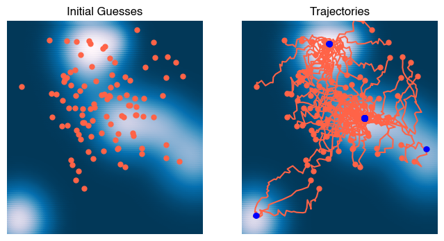
from matplotlib.animation import FuncAnimation
from matplotlib.collections import LineCollection
from IPython.display import HTML

Xs = np.array(optimizer.Xs)[::2][:500]

fig, ax = plt.subplots(figsize=(6, 6))
# ax.scatter(X[:, 0], X[:, 1], c=Z, s=14, zorder=0)
plt.imshow(Z.reshape(100, 100), extent=[-3, 3, -3, 3], origin='lower')
ax.plot(Xs[0, :, 0], Xs[0, :, 1], '.', ms=6, linestyle='None', zorder=1)
curr = ax.scatter([], [], s=20, c='b', zorder=3)
trail = LineCollection([], zorder=2)
ax.add_collection(trail)

ax.set_xlim(-3, 3); ax.set_ylim(-3, 3); ax.axis('off')
plt.margins(0, 0); plt.gca().xaxis.set_major_locator(plt.NullLocator())
plt.gca().yaxis.set_major_locator(plt.NullLocator())

def init():
    curr.set_offsets(np.array([0, 0]))
    trail.set_segments([])
    return (curr, trail)

def update(t):
    # current points
    curr.set_offsets(Xs[t])

    if t > 0:
        segs = []
        # Build one polyline per particle (skip if fewer than 2 points)
        for n in range(Xs.shape[1]):
            path = Xs[:t+1, n, :]  # (k,2)
            if path.shape[0] >= 2:
                segs.append(path)
        trail.set_segments(segs)


    return (curr, trail)

ani = FuncAnimation(fig, update, frames=min(500, Xs.shape[0]),
                    init_func=init, interval=100, blit=True, repeat=True)
html = ani.to_html5_video()                                 # replaces to_jshtml()
HTML(html)
We can see that the Metropolis algorithm is able to find the global minimum of the loss landscape. Qualitatively, the dynamics resemble a random walk in the “flat” regions of the loss landscape, where the acceptance/rejection of a given random move is entirely determined by the Boltzmann factor. However, once the system finds a well, the landscape geometry begins to dominate the dynamics, and the system converges to the minimum.
Since the optimizer is sensitive to the local gradient in the landscape, it uses a form of coarse gradient information because it compares the energy of the current and proposed configurations.
Hard sphere packing and the jamming transition
A basic problem in materials science, statistical physics, and the theory of disordered systems is to find the densest possible packing of hard spheres in a finite volume. Given some fixed volume in dimensions, how many spheres of uniform radius can we fit into it? This problem maps onto many basic phenomena in materials science, such as the freezing transition, bridging continuum and atomistic descriptions of materials, and the behavior of granular materials and glasses.
Here, we will focus on the jamming transition, which is the transition from a fluid to a solid state.
The control parameter for this transition is the packing fraction , which is the fraction of the total volume that is occupied by the spheres. We can think of the packing fraction as a dimensionless measure of the density of the system.
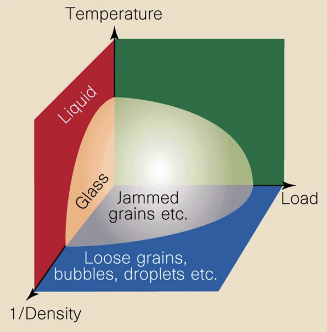
A schematic of the phase diagram for jamming as a function of the inverse density, temperature, and load applied to the entire system. In packing problems, the packing fraction acts as a nondimensional density. From Liu and Nagel, 1998.
Jamming in two dimensions
Here, we will focus on the two-dimensional case of packing hard disks into a square domain. We define a “hard” sphere as a sphere of radius that cannot overlap with any other sphere. The packing fraction is the fraction of the total volume that is occupied by the spheres. In two dimensions, this is given by
where is the number of spheres in our system, is the volume of the domain, and is the radius of each sphere.
The energy of this system is given by the sum of the pairwise potential energy between all pairs of spheres,
where is the distance between the centers of the spheres and is the interaction energy between two spheres. We will consider the case of hard spheres, where the interaction energy is infinite for and zero for .
where is the distance between the centers of the spheres and is the radius of each sphere. Because the system’s total energy is a sum over all pairs of spheres, the total energy is also either 0 (if no two spheres overlap) or (if any two spheres overlap).
class HardDiskPacking:
    """
    Metropolis Monte Carlo for hard disks in 2D with periodic boundaries (unit square).

    Args:
        n (int): Number of particles.
        phi (float): Areal packing fraction (sum of disk areas / box area).
        zeta (float): Maximum trial displacement magnitude (in box-length units).
        store_history (bool): If True, stores coordinates after each sweep.

    Attributes:
        coords (np.ndarray): (N,2) array of particle centers in [0,1)×[0,1).
        diameter (float): Disk diameter implied by (n, phi) in a unit-area box.
        acceptance_rate (float): Fraction of accepted trial moves.
        history (list[np.ndarray] | None): Optional trajectory snapshots.
    """

    def __init__(self, n, phi, store_history=False):
        self.N = int(n)
        self.phi = float(phi)
        self.store_history = bool(store_history)

        # Square lattice initialization in the unit square
        self.coords = self._initialize_lattice()

        # For 2D: phi = N * (pi/4) * d^2  (box area = 1)  ⇒ d = sqrt(4*phi/(pi*N))
        self.diameter = np.sqrt(4.0 * self.phi / (np.pi * self.N))
        # Back-compat with original naming if downstream code expects "radius"
        self.radius = self.diameter

        self.acceptance_rate = None
        if self.store_history:
            self.history = [self.coords.copy()]

    def _initialize_lattice(self):
        """Square mesh in [0,1)^2 with the first N points taken."""
        nx = ny = int(np.ceil(self.N**0.5))
        x = np.linspace(0.0, 1.0, nx, endpoint=False)
        y = np.linspace(0.0, 1.0, ny, endpoint=False)
        xx, yy = np.meshgrid(x, y, indexing="ij")
        coords = np.column_stack((xx.ravel(), yy.ravel()))
        return coords[:self.N].copy()
We can break this class down into a few different components. First, we need to initialize a set of particles within the square volume. We need to make sure that the initial configuration is a valid configuration, which means that no two particles overlap. We can do this by placing the particles in a square lattice. In order to achieve a controllable packing fraction , our code accepts and as input, and internally scales the particle radius to achieve the desired packing fraction,
hdp = HardDiskPacking(100, 0.5, store_history=True)

fig, ax = plt.subplots()
ec = make_ellipses(hdp.coords, hdp.radius / 2, ax=ax)
ec.set_animated(True)
ax.add_collection(ec)
ax.set_xlim(0 - hdp.radius / 2, 1 + hdp.radius / 2); ax.set_ylim(0 - hdp.radius / 2, 1 + hdp.radius / 2)
ax.set_aspect('equal', adjustable='box')
plt.title(f"Initial configuration with {hdp.N} particles and packing fraction {hdp.phi}");

Next, we need to implement boundary conditions for our lattice. Usually, we are interested in systems in the limit of many degrees of freedom (in our case, many particles), and so we want to minimize finite-size effects in our simulations. We can do this by using periodic boundary conditions. There are several ways to implement this, including defining redefining the distance in our simulation domain so that distances are computed modulo the side length of the box. However, this is a bit tricky to do in practice, so we will use a simpler approach (albeit one that requires more memory) simply by replicating the simulation box on all sides.
from scipy.spatial.distance import pdist
import itertools


def augment_lattice(coords):
    """
    Given a set of 2D coordinates, build an augmented lattice of coordinates by
    shifting each coordinate by 1 in each direction around the simulation box
    (assumed to be a unit square).

    Args:
        coords (np.ndarray): coordinates of the particles of shape (N, 2)

    Returns:
        np.ndarray: augmented coordinates of shape (8 * N, 2)
    """
    coords_augmented = list()
    # there are 8 possible shifts to fully surround a simulation box with
    # replicates to create boundary conditions.
    for shift in itertools.product([-1., 0., 1.], repeat=2):
        # if np.sum(np.abs(shift)) == 0:
            # continue # Skip the zero shift case, which is the identity
        coords_augmented.append(coords.copy() + np.array(shift))
    return np.vstack(coords_augmented).copy()
hdp = HardDiskPacking(100, 0.7, store_history=True)
fig, ax = plt.subplots()
ec = make_ellipses(augment_lattice(hdp.coords), hdp.radius / 2, ax=ax)
ec.set_animated(True)
ax.add_collection(ec)
# ax.set_xlim(0 - hdp.radius / 2, 1 + hdp.radius / 2); ax.set_ylim(0 - hdp.radius / 2, 1 + hdp.radius / 2)
ax.set_xlim(-0.5, 1.5); ax.set_ylim(-0.5, 1.5)
ax.set_aspect('equal', adjustable='box')
plt.title(f"Initial configuration with {hdp.N} particles and packing fraction {hdp.phi}");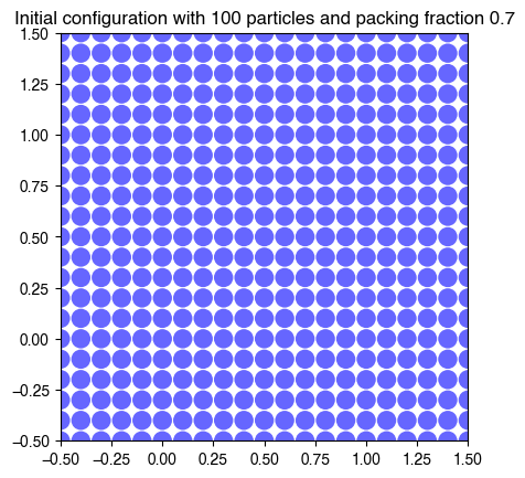
We are now ready to implement the Metropolis Monte Carlo algorithm for a hard disk system.
We take the current configuration of the simulation box (the set of all particle locations) as our starting configuration.
We propose a new configuration by randomly displacing a single particle by a small amount.
We calculate the energy of the new configuration. Recall that, in traditional Metropolis, we calculate the ratio of the Boltzmann factors for the current and proposed configurations:
For the hard disk system, the energy is either 0 or , depending on whether the proposed move causes an overlap between two spheres. As a result, is either 1 or 0, depending on whether the proposed move causes an overlap between two spheres. This means that the acceptance probability is either 1 or 0, and we can simply accept or reject the proposed move based on whether the proposal causes an overlap between two spheres. The hyperparameter therefore vanishes from the Metropolis scheme for this system.
We accept the new configuration with probability 1 if it has no overlaps, and with probability 0 if it has overlaps.
Thus, in order to perform a Metropolis Monte Carlo simulation for the hard disk system, we need only check whether a proposed move causes an overlap between any two spheres. If it does, we reject the move, and if it doesn’t, we accept the move. We therefore implement a function that finds the pairwise distances between all particles in the simulation box, and checks whether any of those distances are less than twice the radius of the particles.
def has_overlaps(coords, i, radius):
    """
    Check if particle i overlaps any other using the minimum-image convention.

    Overlap criterion: |r_i - r_j| < diameter.
    """
    coords = augment_lattice(coords)
    # Displacements to all particles
    disp = coords[i] - coords
    # Minimum-image in a unit box (maps to [-0.5,0.5))
    disp -= np.rint(disp)
    # Distances; exclude self (zero distance)
    dists = np.hypot(disp[:, 0], disp[:, 1])
    dists = dists[dists > 0.0]
    return np.any(dists < radius)
We can now try initializing the hard disk system and proposing a single update move, to see if our function for checking for overlaps is working.
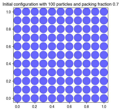
hdp = HardDiskPacking(100, 0.7, store_history=True)
fig, ax = plt.subplots()
ec = make_ellipses(augment_lattice(hdp.coords), hdp.radius / 2, ax=ax)
ec.set_animated(True)
ax.add_collection(ec)
ax.set_xlim(0 - hdp.radius / 2, 1 + hdp.radius / 2); ax.set_ylim(0 - hdp.radius / 2, 1 + hdp.radius / 2)
ax.set_aspect('equal', adjustable='box')
plt.title(f"Initial configuration with {hdp.N} particles and packing fraction {hdp.phi}");
print("Proposed configuration has overlaps:", has_overlaps(hdp.coords, 55, hdp.radius))
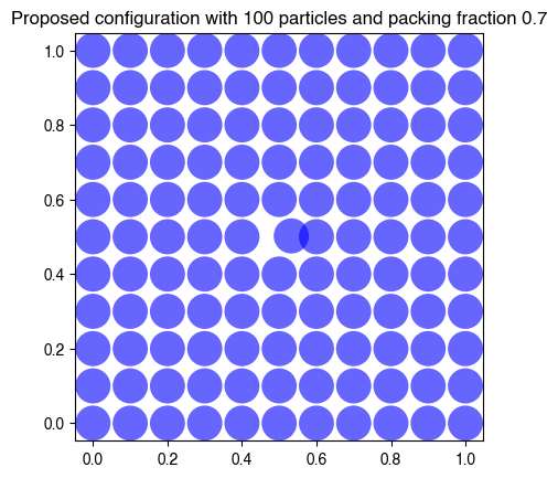
### propose a new configuration
hdp.coords[55] = hdp.coords[55] + 0.04 * (2 * np.random.rand(2) - 1)
fig, ax = plt.subplots()
ec = make_ellipses(augment_lattice(hdp.coords), hdp.radius / 2, ax=ax)
ec.set_animated(True)
ax.add_collection(ec)
ax.set_xlim(0 - hdp.radius / 2, 1 + hdp.radius / 2); ax.set_ylim(0 - hdp.radius / 2, 1 + hdp.radius / 2)
# ax.set_xlim(-0.5, 1.5); ax.set_ylim(-0.5, 1.5)
ax.set_aspect('equal', adjustable='box')
plt.title(f"Proposed configuration with {hdp.N} particles and packing fraction {hdp.phi}");
print("Proposed configuration has overlaps:", has_overlaps(hdp.coords, 55, hdp.radius))
Proposed configuration has overlaps: False
Proposed configuration has overlaps: True
We are now ready to add a method that performs the full Metropolis Monte Carlo simulation. We subclass our HardDiskPacking class to add a fit method that performs the Metropolis Monte Carlo simulation. does not appear as a hyperparameter, because the acceptance criterion is fully deterministic (whether or not a proposed move is accepted is fully determined by whether it causes an overlap between two spheres). However, we do need to specify a maximum trial displacement hyperparameter , which controls the size of the random displacements used to perturb the current configuration.
class HardDiskMonteCarlo(HardDiskPacking):
    """
    Metropolis Monte Carlo for hard disks in 2D with periodic boundaries (unit square).

    Args:
        n (int): Number of particles.
        phi (float): Areal packing fraction (sum of disk areas / box area).
        store_history (bool): If True, stores coordinates after each sweep.
        zeta (float): Maximum trial displacement magnitude (in box-length units).

    Attributes:
        coords (np.ndarray): (N,2) array of particle centers in [0,1) x [0,1).
        diameter (float): Disk diameter implied by (n, phi) in a unit-area box.
        acceptance_rate (float): Fraction of accepted trial moves.
        history (list[np.ndarray] | None): Optional trajectory snapshots.
    """

    def __init__(self, *args, zeta=0.01, **kwargs):
        super().__init__(*args, **kwargs)
        self.zeta = zeta

    def fit(self, num_iter=1000, verbose=False):
        """
        Run num_iter Monte Carlo sweeps (each sweep: N single-particle trials).

        Args:
            num_iter (int): Number of sweeps.
            verbose (bool): Print progress every 50 sweeps.

        Returns:
            self
        """
        accepts, rejects = 0, 0

        for it in range(num_iter):
            for j in range(self.N):
                trial = self.coords.copy()
                # Random displacement in 2D within [-zeta, zeta]^2
                trial[j] = (trial[j] + self.zeta * (2.0 * np.random.rand(2) - 1.0)) % 1.0

                if not has_overlaps(trial, j, self.radius):
                    self.coords[j] = trial[j]
                    accepts += 1
                else:
                    # if np.random.rand() < 0.1:
                    #     self.coords[j] = trial[j]
                    rejects += 1

            if verbose and (it % 50 == 0):
                print(f"sweep {it}")

            if self.store_history:
                self.history.append(self.coords.copy())

        self.acceptance_rate = accepts / (accepts + rejects) if (accepts + rejects) else 0.0
        return self
Notice that we implemented our hard disk Monte Carlo algorithm as a subclass of our HardDiskPacking class. Since the acceptance criterion depends on geometric parameters, we want the simulation to have access to all of the attributes associated with the original system.
We are now ready to run a full simulation.
## Run simulation

hdp = HardDiskMonteCarlo(100, 0.2, zeta=0.01, store_history=True)

hdp.fit(num_iter=500, verbose=True)

print(f"Terminated Metropolis with average acceptance rate {hdp.acceptance_rate}")
sweep 0
sweep 50
sweep 100
sweep 150
sweep 200
sweep 250
sweep 300
sweep 350
sweep 400
sweep 450
Terminated Metropolis with average acceptance rate 0.90158
plt.figure()
init_coords = hdp.history[0]
final_coords = hdp.history[-1]

plt.figure(figsize=(10, 5))
ax1 = plt.subplot(1, 2, 1)
ec = make_ellipses(init_coords, hdp.radius / 2, ax=ax1)
# ec.set_animated(True)
ax1.add_collection(ec)
ax1.set_xlim(0 - hdp.radius / 2, 1 + hdp.radius / 2); ax1.set_ylim(0 - hdp.radius / 2, 1 + hdp.radius / 2)
ax1.set_aspect('equal', adjustable='box')
ax1.set_title(f"Initial configuration at packing fraction {hdp.phi}");

ax2 = plt.subplot(1, 2, 2)
ec = make_ellipses(final_coords, hdp.radius / 2, ax=ax2)
ax2.add_collection(ec)
ax2.set_xlim(0 - hdp.radius / 2, 1 + hdp.radius / 2); ax2.set_ylim(0 - hdp.radius / 2, 1 + hdp.radius / 2)
ax2.set_aspect('equal', adjustable='box')
ax2.set_title(f"Final configuration at packing fraction {hdp.phi}");
<Figure size 640x480 with 0 Axes>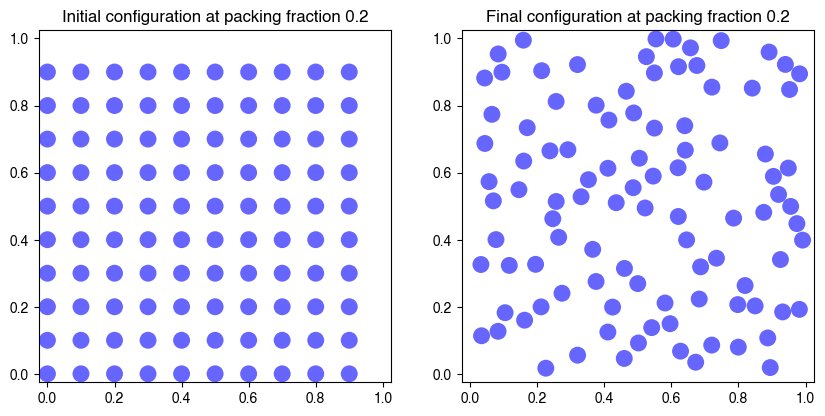
import numpy as np

import matplotlib.pyplot as plt
from matplotlib.animation import FuncAnimation, FFMpegWriter, PillowWriter
from IPython.display import HTML
import shutil

# from matplotlib.collections import EllipseCollection
# def make_ellipses(coords, r):
#     w0 = np.full(len(coords), 2*r)
#     h0 = np.full(len(coords), 2*r)
#     ec = EllipseCollection(
#         w0, h0, np.zeros(len(coords)),
#         units='xy',                      # widths/heights are in data units
#         offsets=coords, offset_transform=ax.transData,
#         facecolor='b', edgecolor='none', alpha=0.6
#     )
#     return ec

def make_video_from_history(hdp, interval=100, repeat=True, save_path=None, r=0.1):
    """
    Args:
        hdp: Object with attribute `history` that is an indexable sequence where each
            element is an (N, 2) array of point coordinates for that frame.
        interval (int): Delay between frames in milliseconds.
        repeat (bool): Whether the animation repeats when finished.
        save_path (str or None): If provided (e.g., 'out.mp4' or 'out.gif'), the animation
            will be written to this file.
        r (float): Circle radius in *data/axis* units.

    Returns:
        (matplotlib.animation.FuncAnimation): The animation object (also displayable via HTML()).
    """
    frames = len(hdp.history)
    if frames == 0:
        raise ValueError("hdp.history appears to be empty.")

    # Initial frame
    coords0 = np.asarray(hdp.history[0])
    coords0 = augment_lattice(coords0)
    if coords0.ndim != 2 or coords0.shape[1] != 2:
        raise ValueError("Each entry of hdp.history must be an (N, 2) array of coordinates.")

    fig, ax = plt.subplots(figsize=(8, 8))

    # --- EllipseCollection in *data units* (width/height are 2*r) ---
    # w0 = np.full(len(coords0), 2*r)
    # h0 = np.full(len(coords0), 2*r)
    # ec = EllipseCollection(
    #     w0, h0, np.zeros(len(coords0)),
    #     units='xy',                      # widths/heights are in data units
    #     offsets=coords0, offset_transform=ax.transData,
    #     facecolor='b', edgecolor='none', alpha=0.6
    # )
    ec = make_ellipses(coords0, r, ax=ax)
    ec.set_animated(True)               # better blitting
    ax.add_collection(ec)

    # Axes housekeeping
    ax.set_xlim(0, 1); ax.set_ylim(0, 1)
    ax.set_aspect('equal', adjustable='box')

    # Track current number of ellipses so we can adjust if N varies by frame
    state = {"n": len(coords0)}

    def _ensure_sizes(n):
        """Resize widths/heights arrays if N changes across frames."""
        if n != state["n"]:
            ec.set_widths(np.full(n, 2*r))
            ec.set_heights(np.full(n, 2*r))
            ec.set_angles(np.zeros(n))
            state["n"] = n

    def init():
        ec.set_offsets(coords0)
        _ensure_sizes(len(coords0))
        return (ec,)

    def update(t):
        pts = np.asarray(hdp.history[t])
        pts = augment_lattice(pts)
        _ensure_sizes(len(pts))
        ec.set_offsets(pts)
        return (ec,)

    ani = FuncAnimation(
        fig, update, frames=frames, init_func=init,
        interval=interval, blit=True, repeat=repeat
    )

    # Optional save
    if save_path is not None:
        fps = max(1, int(1000 / interval))
        if save_path.lower().endswith(".gif"):
            ani.save(save_path, writer=PillowWriter(fps=fps))
        else:
            if shutil.which("ffmpeg") is not None:
                ani.save(save_path, writer=FFMpegWriter(fps=fps, bitrate=1800))
            else:
                fallback = save_path.rsplit(".", 1)[0] + ".gif"
                ani.save(fallback, writer=PillowWriter(fps=fps))
                print(f"ffmpeg not found. Saved GIF instead at: {fallback}")

    return ani

ani = make_video_from_history(hdp, interval=100, repeat=True, r=hdp.radius/2);
HTML(ani.to_html5_video())

We can see what happens in this system. At low packing fractions the particles move around freely, only occasionally colliding with one another. However, as the packing fraction grows, a lower fraction of moves get accepted because the particles are caged in, fewer possible motions. Even though we initialize the system in a square configuration, we can see that, at high packing fractions, it approaches hexagonal ordering, which is a slightly denser packing. In fact, hexagonal ordering is the densest possible packing at .
What happens as we vary the packing fraction?
We repeat our experiment from before, but this time we vary the packing fraction.
phi_range = np.linspace(0.01, 0.9, 10)

final_coords = list()
for phi in phi_range:
    hdp = HardDiskPacking(400, phi, zeta=0.01, store_history=True)
    hdp.fit(num_iter=1000, verbose=False)
    print(f"At packing fraction {phi}, Metropolis had average acceptance rate {hdp.acceptance_rate}")

    coords = hdp.history[-1]
    final_coords.append(coords.copy())
At packing fraction 0.01, Metropolis had average acceptance rate 0.97111
At packing fraction 0.10888888888888888, Metropolis had average acceptance rate 0.8749425
At packing fraction 0.20777777777777778, Metropolis had average acceptance rate 0.8048475
At packing fraction 0.30666666666666664, Metropolis had average acceptance rate 0.7180275
At packing fraction 0.40555555555555556, Metropolis had average acceptance rate 0.6138825
At packing fraction 0.5044444444444445, Metropolis had average acceptance rate 0.4831475
At packing fraction 0.6033333333333333, Metropolis had average acceptance rate 0.3227825
At packing fraction 0.7022222222222222, Metropolis had average acceptance rate 0.1409175
At packing fraction 0.8011111111111111, Metropolis had average acceptance rate 0.0
At packing fraction 0.9, Metropolis had average acceptance rate 0.0
We can see the onset of this jammed state by looking at the acceptance ratio as a function of packing fraction. As the packing fraction approaches 0.91, the fraction of accepted proposals drops to zero because there are no valid configurations.
The pairwise correlation function
How do we measure the approach to the jammed state as we vary the packing fraction? One way is to look at the pairwise correlation function, which is a measure of the average number of particles at a given distance from any other particle. The pairwise correlation function is defined as the probability of finding a particle at a distance from another particle, given that the other particle is at the origin. It is given by
where is the overall number density of particles. The sum over excludes the term, which would be infinite. The delta function ensures that the sum is only over pairs of particles that are separated by a distance . The factor of ensures that the sum is normalized by the number of particles, while the factor of ensures that the sum is normalized by the volume of the system. Essentially, this function measures how often, on average, I expect to find a particle at a distance from the center of a given particle, averaged over many particles. However, this function is scaled by the mean density of the system, so that the value of the function approaches one as .
For finite-size systems, as defined here appears “spiky,” comprising a series corresponding to all possible pairs of particles. In the thermodynamic limit, however, the spikes become infinitely narrow and the function becomes smooth. In order to estimate for a finite-size system, we must smooth the function by binning it. We will use a bin size of . In this case, the correlation function is given by
where is the Heaviside step function. The factor of ensures that the sum is normalized by the bin size.
from scipy.spatial.distance import cdist

def compute_g2(coords, nbins=180, rmax=0.5):
    """
    Pair correlation g(r) in 2D. If the average density is not known in advance,
    estimate it from the tail average.

    Args:
        coords (np.ndarray): Coordinates of the particles (N, 2).
        nbins (int): Number of histogram bins (edges returned; g2 has nbins-1).
        rmax (float): Max separation considered.

    Returns:
        bins (np.ndarray): Bin edges (length nbins).
        g2 (np.ndarray): Pair correlation values (length nbins-1).
    """
    D = cdist(coords, coords)  # pairwise distances
    bins = np.linspace(0, rmax, nbins)
    hist, bins = np.histogram(D, bins=bins)

    # 2D shell area: π (r_{k+1}^2 - r_k^2)
    shell_area = np.pi * (bins[1:]**2 - bins[:-1]**2)
    g2 = hist / (len(coords) * shell_area)

    # Optional: normalize by tail average
    g2 = g2 / g2[-3:].mean()
    g2[0] = 0 # Get rid of self term
    return bins, g2
hdp = HardDiskMonteCarlo(200, 0.7, zeta=0.02, store_history=True)
# hdp = HardDiskPacking(200, 0.7, zeta=0.02, store_history=True)
# hdp = HardDiskPacking(500, 0.7, zeta=0.02, store_history=True)
hdp.fit(num_iter=2000, verbose=True)
packing_coords = hdp.history[-1]


bins, hist = compute_g2(augment_lattice(packing_coords), nbins=200)
plt.figure()
plt.plot(bins[:-1], hist, 'k')
plt.xlabel(r'r')
plt.ylabel(r'$g_2(r)$')

# plt.figure()
# fig = plt.figure()
# plt_sphere(hsp.history[1].copy(), hsp.radius)
# plt.xlim([-0.5, 0.5])
# plt.ylim([-0.5, 0.5])
# plt.gca().set_zlim([-0.5, 0.5])

# fig = plt.figure()
# plt_sphere(hsp.history[-1].copy(), hsp.radius),
# plt.xlim([-0.5, 0.5])
# plt.ylim([-0.5, 0.5])
# plt.gca().set_zlim([-0.5, 0.5])
sweep 0
sweep 50
sweep 100
sweep 150
sweep 200
sweep 250
sweep 300
sweep 350
sweep 400
sweep 450
sweep 500
sweep 550
sweep 600
sweep 650
sweep 700
sweep 750
sweep 800
sweep 850
sweep 900
sweep 950
sweep 1000
sweep 1050
sweep 1100
sweep 1150
sweep 1200
sweep 1250
sweep 1300
sweep 1350
sweep 1400
sweep 1450
sweep 1500
sweep 1550
sweep 1600
sweep 1650
sweep 1700
sweep 1750
sweep 1800
sweep 1850
sweep 1900
sweep 1950
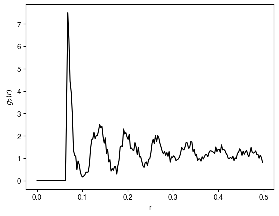
We can compare our results to the typical appearance of the correlation function for a dense packing of hard spheres. The correlation function is a smooth function that decays to one (the asymptotic average density) at long distances.
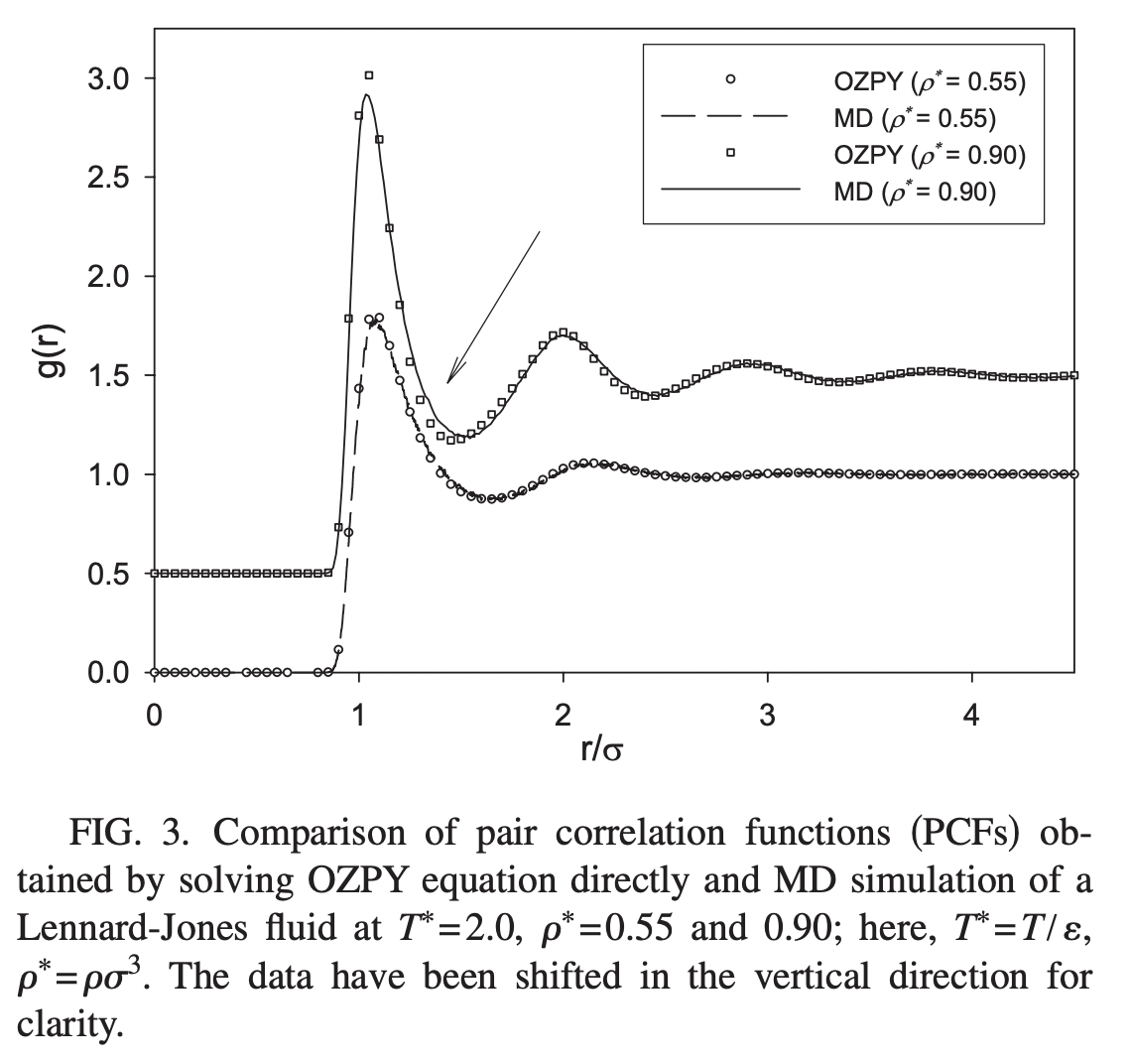
The correlation function computed from molecular dynamics simulations, as well as an analytic approximate solution for g(r). Image from Wang et al. PRE 2010*
Questions
We have a double loop: an outer loop over all iterations, and an inner loop where we go over each individual particle, jostle it, and check for overlaps. Why can’t this inner loop be vectorized?
How would we generalize this approach to a soft-repulsive potential?
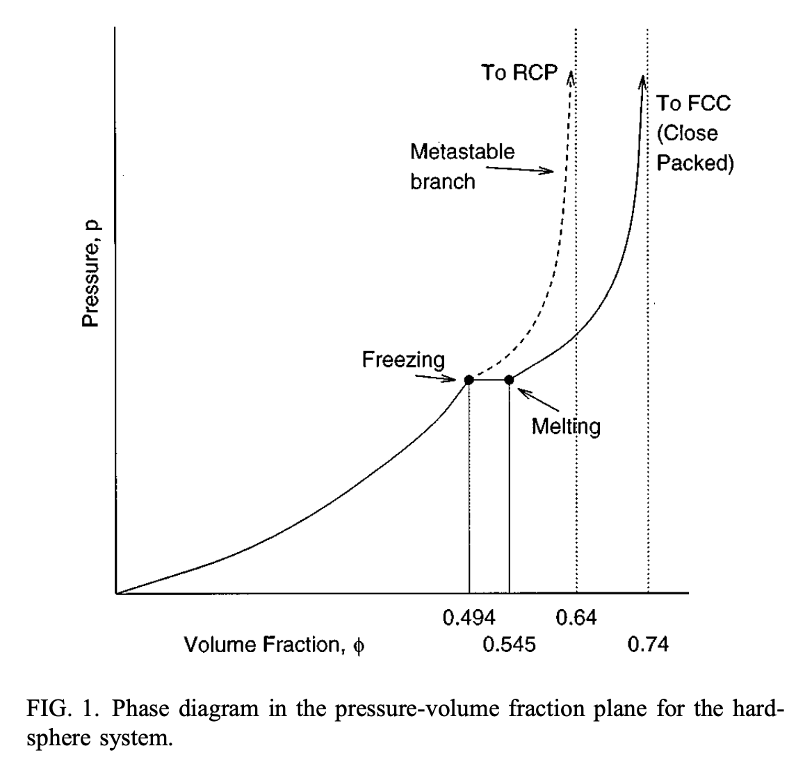
Image from Rintoul & Torquato. JCP 1996
Soft sphere packing
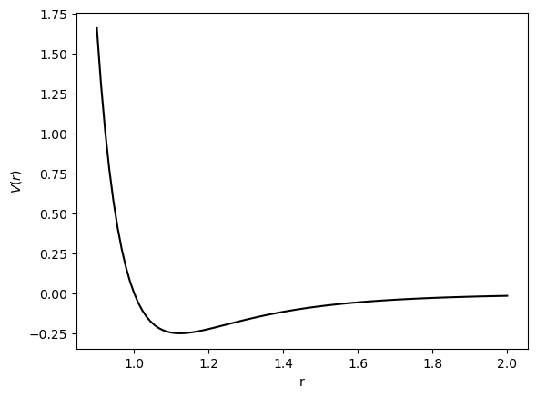
We saw before that the hard-sphere system is a highly simplified model, for which the Monte Carlo update becomes deterministic. We can make the system more realistic by introducing the Lennard-Jones potential.
where is the distance between the centers of the two particles. This corresponds to a soft-repulsive potential that is infinite at contact, and zero at infinite separation. The parameter is the hard-core diameter, and is the depth of the potential well.
In order to implement this potential, we will need to modify the overlap energy function to compute the distance among all pairs of particles, and then calculate their pairwise energies. We then need to sum these energies to get the total energy of a proposal. Finally, we will need to introduce a traditional Monte Carlo acceptance step, parameterized by the inverse temperature hyperparameter .
def lennard_jones(r, sigma=1.0, v0=1.0, tol=1e-6):
    """The Lennard-Jones potential with a small tolerance to avoid division by zero."""
    return v0 * (sigma / (r + tol))**12 - v0 * (sigma / (r + tol))**6

rvals = np.linspace(0.9, 2, 100)
plt.figure()
plt.plot(rvals, lennard_jones(rvals), 'k')
plt.xlabel(r'r')
plt.ylabel(r'$V(r)$')
plt.show()
from scipy.spatial.distance import cdist

class SoftDiskPacking(HardDiskPacking):
    """
    Metropolis Monte Carlo for hard disks in 2D with periodic boundaries (unit square).

    Args:
        n (int): Number of particles.
        phi (float): Areal packing fraction (sum of disk areas / box area).
        softness (float): The frequency of accepting overlaps
        zeta (float): Maximum trial displacement magnitude (in box-length units).
        store_history (bool): If True, stores coordinates after each sweep.

    Attributes:
        coords (np.ndarray): (N,2) array of particle centers in [0,1)×[0,1).
        diameter (float): Disk diameter implied by (n, phi) in a unit-area box.
        acceptance_rate (float): Fraction of accepted trial moves.
        history (list[np.ndarray] | None): Optional trajectory snapshots.
    """

    def __init__(self, n, phi, beta=1.0, **kwargs):
        super().__init__(n, phi, **kwargs)
        self.beta = beta

    def overlap_energy(self, coords):
        """
        Compute the overlap energy of a configuration of disks.
        """
        D = cdist(coords, coords) # pairwise distances
        ## exclude self-interaction
        np.fill_diagonal(D, np.inf)
        pairwise_energies = lennard_jones(D, sigma=self.radius)
        return np.sum(pairwise_energies)

    def fit(self, num_iter=1000, verbose=False):
        """
        Run num_iter Monte Carlo sweeps (each sweep: N single-particle trials).

        Args:
            num_iter (int): Number of sweeps.
            verbose (bool): Print progress every 50 sweeps.

        Returns:
            self
        """
        accepts, rejects = 0, 0

        for it in range(num_iter):

            ## Iterate over all particles
            for j in range(self.N):

                ## Perturbation is a random displacement in 2D within [-zeta, zeta]
                trial = self.coords.copy()
                trial[j] = (trial[j] + self.zeta * (2.0 * np.random.rand(2) - 1.0)) % 1.0
                trial_energy = self.overlap_energy(trial)
                current_energy = self.overlap_energy(self.coords)
                delta_energy = trial_energy - current_energy
                accept_higher = np.random.uniform() < np.exp(-delta_energy * self.beta)

                if delta_energy < 0 or accept_higher:
                    self.coords[j] = trial[j]
                    accepts += 1
                else:
                    rejects += 1

            if verbose and (it % 50 == 0):
                print(f"sweep {it}, cumulative acceptance rate {accepts / (accepts + rejects)}")

            if self.store_history:
                self.history.append(self.coords.copy())

        self.acceptance_rate = accepts / (accepts + rejects) if (accepts + rejects) else 0.0
        return self
hdp = SoftDiskPacking(100, 0.85, beta=1e0, zeta=0.01, store_history=True)

hdp.fit(num_iter=500, verbose=True)
## Save the history because this simulation is demanding
# np.savez('../private_resources/monte_carlo_metropolis.npz', np.array(hsp.history))

print(f"Terminated Metropolis with average acceptance rate {hdp.acceptance_rate}")
sweep 0, cumulative acceptance rate 0.25
sweep 50, cumulative acceptance rate 0.38666666666666666
sweep 100, cumulative acceptance rate 0.4266336633663366
sweep 150, cumulative acceptance rate 0.4506622516556291
sweep 200, cumulative acceptance rate 0.46800995024875625
sweep 250, cumulative acceptance rate 0.4806772908366534
sweep 300, cumulative acceptance rate 0.48727574750830566
sweep 350, cumulative acceptance rate 0.4943019943019943
sweep 400, cumulative acceptance rate 0.500573566084788
sweep 450, cumulative acceptance rate 0.5061862527716187
Terminated Metropolis with average acceptance rate 0.50868
## Run simulation
ani = make_video_from_history(hdp, interval=100, repeat=True, r=hdp.radius/2)
HTML(ani.to_html5_video())
packing_coords = hdp.history[-1]
bins, hist = compute_g2(augment_lattice(packing_coords), nbins=200)
plt.figure()
plt.plot(bins[:-1], hist, 'k')
plt.xlabel(r'r')
plt.ylabel(r'$g_2(r)$')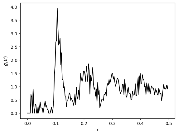
What about cost?
For both the hard-sphere and soft-sphere systems, we queried the the energy of a proposed update by calculating the pairwise distances among all pairs of particles. In optimization, the runtime is usually bottlenecked by the number of calls to the energy function. Here, computing all possible pairwise distances introduces a cost of to compute a single proposal. As a result, our procedure for simulating interacting particles scales poorly to high-dimensional systems. In practice, if we want to recreate continuum theories of interacting particles, we need to find ways to reduce the cost of computing the energy function.
Notice how, near the jammed state, a proposed update only affects a small fraction of particles in the immediate vicinity of the particle we are perturbing. For a hard-sphere system, a proposed update of size can only affect the pairwise energy of particles that fall within a distance of the edges of an unperturbeddisk (or from its center of mass). As a result, instead of computing all pairwise distances, to compute the energy change we only need to look up neighbors within a finite spatial radius.
For the Lennard-Jones potential, all particles technically interact with all other particles, because the potential decays to zero at infinite separation. However, the typical interaction range is much smaller than the system size, so we can still reduce the cost of computing the energy function by only considering particles within a finite spatial radius. This is equivalent to truncating the potential at a cutoff distance far beyond the typical interaction range. In general, in Monte Carlo schemes, we can often exploit locality of perturbations to save compute. Another example of this is the Ising model, where a single proposed spin flip only affects the energy through its nearest neighbors.
What about longer-ranged potentials? For example, gravitational interactions fall off as . In this case, truncating the potential might lead to physical effects. In this case, specialized algorithms like the Barnes-Hut algorithm, Ewald summation, or the Fast Multipole Method can be used to compute the energy function more efficiently.
Further reading
A recent modification of the Metropolis algorithm by Muller et al., rearranges the acceptance step
where is a random number between 0 and 1. This approach therefore re-frames the Metropolis update as determining whether the proposed energy change lies above or below the random threshold .
The key insight of Müller et al. is that does not need to be known exactly. Rather, it is sufficient to gradually update a set of upper and lower bounds, . If then the update is accepted. If then the update is rejected probabilistically.
Thus, rather than exactly compute the energy change, the authors can use a tree-like decomposition of the domain to gradually improve bounds on the true energy change, until one of the stopping conditions above is triggered. Importantly, this is an exact algorithm, and it does not require any approximations.
From the Martiniani lab: basins of attraction video for soft repulsive particles
- Liu, A. J., & Nagel, S. R. (1998). Jamming is not just cool any more. Nature, 396(6706), 21–22. 10.1038/23819
- Wang, Q., Keffer, D. J., Nicholson, D. M., & Thomas, J. B. (2010). Use of the Ornstein-Zernike Percus-Yevick equation to extract interaction potentials from pair correlation functions. Physical Review E, 81(6). 10.1103/physreve.81.061204
- Rintoul, M. D., & Torquato, S. (1996). Computer simulations of dense hard-sphere systems. The Journal of Chemical Physics, 105(20), 9258–9265. 10.1063/1.473004
- Müller, F., Christiansen, H., Schnabel, S., & Janke, W. (2023). Fast, Hierarchical, and Adaptive Algorithm for Metropolis Monte Carlo Simulations of Long-Range Interacting Systems. Physical Review X, 13(3). 10.1103/physrevx.13.031006