Python Objects, Optical Traps, and the Ornstein-Uhlenbeck process

In this notebook, we will discover how object-oriented programming allows a level of abstraction that is well-suited for describing physical systems. We will focus on stochastic processes, a broad class of systems that are well described by random variables that change in time. We will use our simulations to study the first passage time distribution, a fundamental concept for understanding how random processes can have predictable ensemble properties.

Open this notebook in Google Colab:

We start by importing the necessary Python packages.

# Import local plotting functions and in-notebook display functions
import matplotlib.pyplot as plt
%matplotlib inline

# Import linear algebra module
import numpy as np

Ornstein-Uhlenbeck processes¶

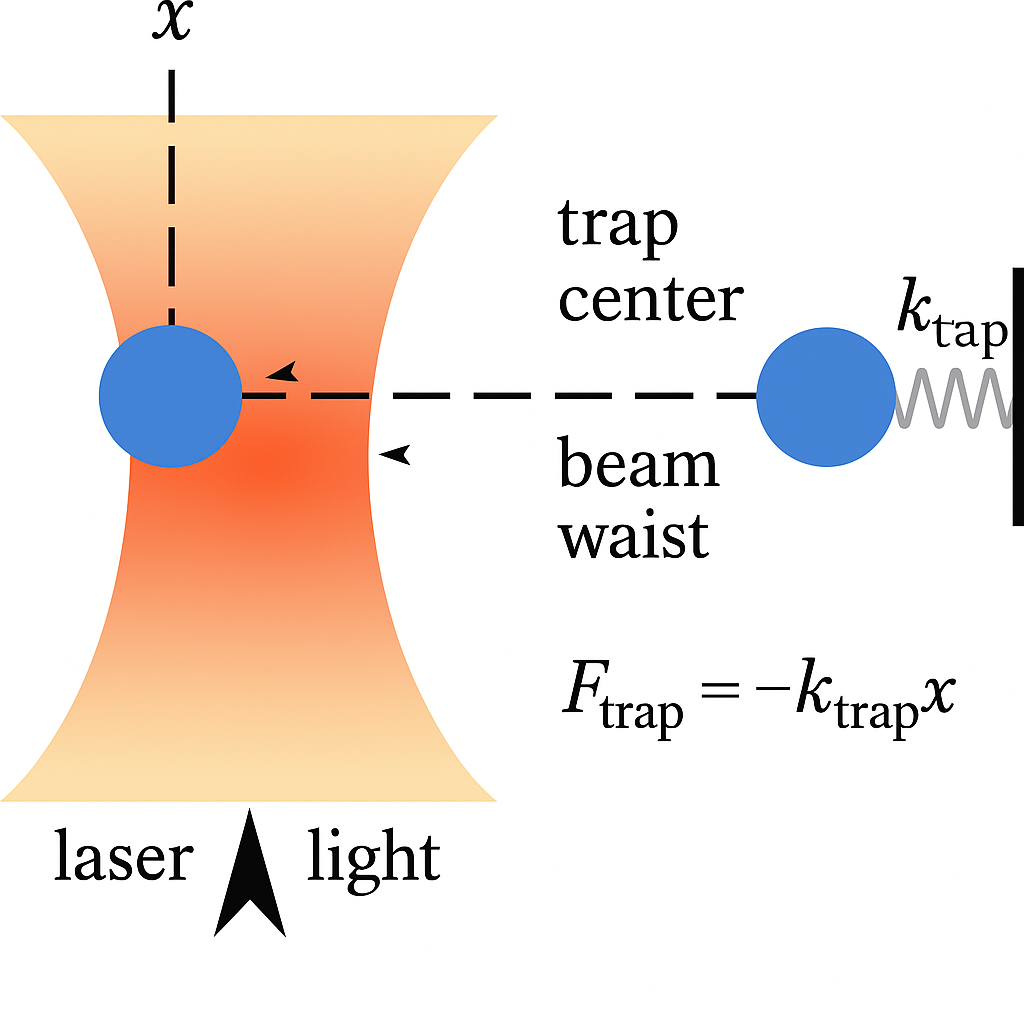
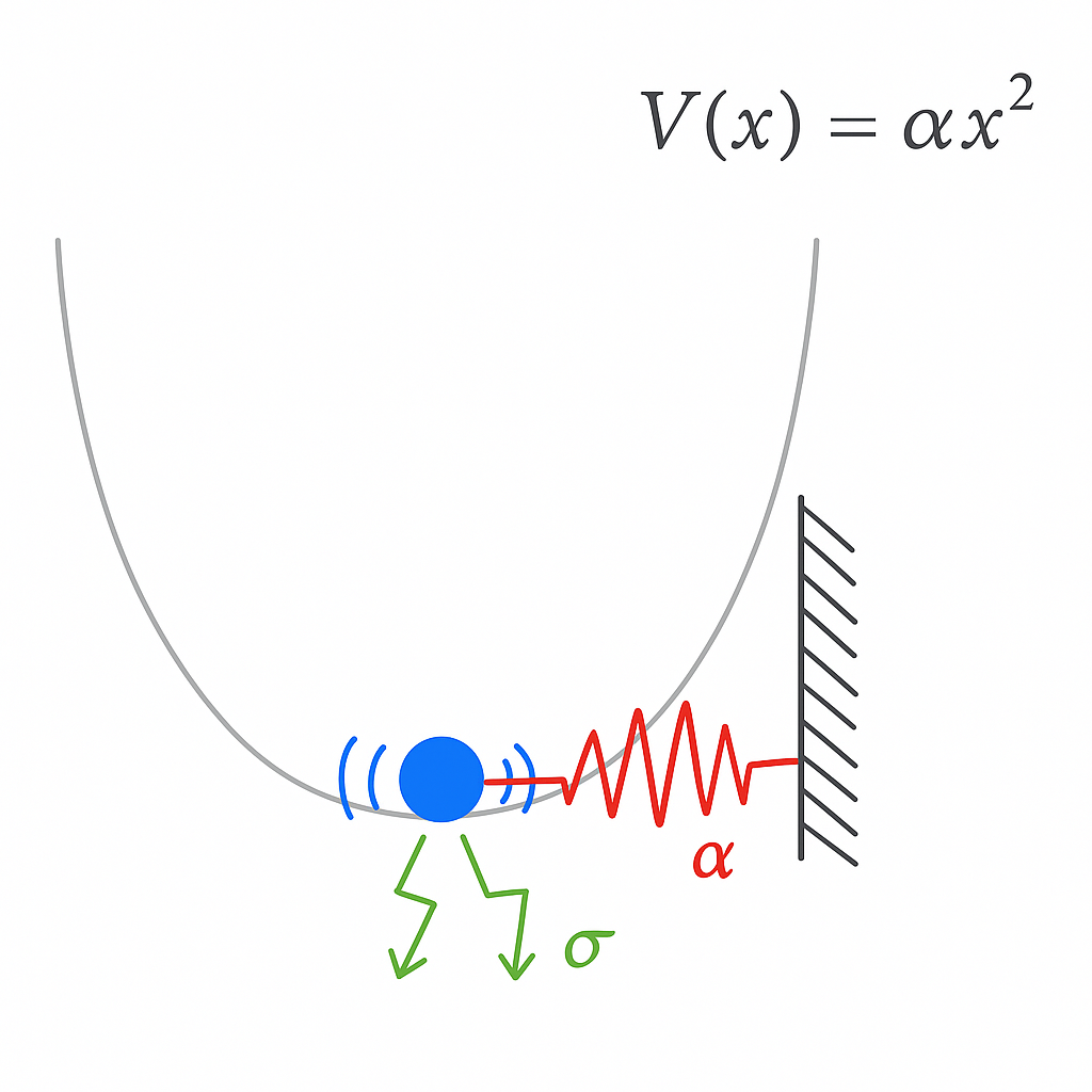
Ornstein-Uhlenbeck processes describe the motion of a particle attached to a simple Hookean spring, in the presence of noise. They are a minimal model of physical systems with a balance of confining forces and stochastic forces.

In biophysics and atomic physics, specialized devices called optical traps are well described by Ornstein-Uhlenbeck processes. Laser light is used to confine a particle near the center of the trap, but the particle jiggles in place due to Brownian forces because its small size.

A nanoparticle (103 nm in diameter) trapped by an optical tweezer. Bjschellenberg, CC BY-SA 4.0 via Wikimedia Commons and Cr4sZz, CC BY-SA 4.0 via Wikimedia Commons

Mathematically, we can describe an Ornstein-Uhlenbeck process by writing a stochastic differential equation,

dx_{t}=-\alpha \,x_{t}\,dt+\sigma \,dW_{t}

(1)

This equation states that the infinitestimal displacement $dx_{t}$ of a particle over a short time interval is partly determined by a restoring force that scales with the spring constant $\alpha$ , the current displacement $x_t$ , and the duration of the interval $dt$ . However, the motion is also driven by a noise term $dW_t$ , which describes a series of random “kicks” to the particle at random times, with characteristic amplitude $\sigma$ .

A tighter, more confining optical trap with have a higher $\alpha$ . Conversely, if we increase the temperature of the air around an optical trap, or decrease the size of the particle we are trapping, we expect that $\sigma$ will increase.

We want to simulate this stochastic process in discrete time. In order to do this, we will pick a specific, fixed time interval $\Delta t$ , and write a difference equation,

x_{t+1}=x_{t}-\alpha \,x_{t}\,\Delta t+\sigma \,\sqrt{\Delta t}\,Z_{t}

(2)

where $Z_{t}$ is a standard normal random variable. Because Brownian forces correspond to a non-differential set of random kicks, they are well modeled by numbers randomly sampled from the normal distribution. However, one complication is that, over longer intervals $\Delta t$ , it becomes possible for a series of random kicks to push the particle further from the center. We can account for this by introducing the scale factor $\sqrt{\Delta t}$ into our discrete-time dynamics.

Because $\Delta t$ appears in both terms in this expression, we can simplify by absorbing it into our two experimental parameters $\alpha$ and $\sigma$ . Physically, this corresponds to measuring time in a set of units for which $\Delta t=1$ .

Python functions¶

Python functions are objects that can be called. They are defined using the def keyword, and can be called using the () syntax.

There are several unique features of Python functions that we will use in this course:

Keyword arguments are optional arguments that accept default values. The default values are used if the argument is not provided when the function is called.
Variables used within functions always have local scope, and are not accessible outside of the function.
Docstrings are used to describe all arguments and returns in human-readable text. They are not used by the Python interpreter, but are used by tools like help() to provide information about the function.
We very often need to use functions that were written by others, in order to define our own functions. For example, we are going to import a library called random, which supports functions for sampling random distributions.

# Import additional modules of the python library, which implement features that we might need
import random
import math

def ornstein_uhlenbeck_process(x, alpha=0.1, sigma=1.0, dt=1.0):
    """
    One step for the dynamics of a particle in a harmonic potential, with Brownian noise

    Equivalent to an AR(1) process with alpha = 1

    Args:
        x (float): The current position of the particle
        alpha (float): The spring constant
        sigma (float): The amplitude of the random noise

    Returns:
        float: The position of the particle at the next time step
    """
    # forcing term
    drift = -alpha * x * dt

    # stochastic diffusion term
    # random.gauss(0, 1) samples a random value from a normal distribution with mean 0 
    # and variance 1
    diffusion = sigma * random.gauss(0, 1) * math.sqrt(dt)

    # The OU process is a combination of drift and diffusion
    x_nxt = x + drift + diffusion
    return x_nxt

Let’s test that our implementation of the Ornstein-Uhlenbeck process is correct. We will create a for loop that runs the process for 400 steps, storing each step in a list that grows as we iterate.

We can repeat the simulation for different values of the confinement strength $\alpha$ and the noise amplitude $\sigma$ , and see how the behavior of the process changes. For each of the experiments, we modify $\alpha$ in different ways, to show the different syntax for passing arguments to functions. Since both $\alpha$ and $\sigma$ are keyword arguments with default values, we can set them directly. We can also pass values directly without naming them, as long as we follow the order of the arguments in the original function signature. We can also mix and match these different syntaxes, as long as we don’t violate the order of the arguments.

all_steps = [0]
for i in range(400):
    all_steps.append(
        ornstein_uhlenbeck_process(all_steps[-1], alpha=0.1, sigma=1)
    )
plt.plot(all_steps, label="alpha=0.5, sigma=1")
plt.xlabel("time")
plt.ylabel("position")

# all_steps = [0]
# for i in range(400):
#     all_steps.append(
#         ornstein_uhlenbeck_process(all_steps[-1], sigma=1, alpha=1)
#     )
# plt.plot(all_steps, label="alpha=1, sigma=1")

# all_steps = [0]
# for i in range(400):
#     all_steps.append(
#         ornstein_uhlenbeck_process(all_steps[-1], 0.0)
#     )
# plt.plot(all_steps, label="alpha=0, sigma=1")

plt.legend(frameon=False)
plt.xlabel("time")
plt.ylabel("position")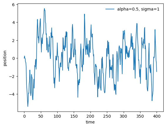

Python also supports an alternative syntax for defining functions, using the lambda keyword. This is useful for short functions with simple behavior.


ornstein_uhlenbeck_process_alternate = lambda x, alpha=0.5, sigma=1.0, dt=1.0: x - alpha * x * dt+ sigma * random.gauss(0, 1) * math.sqrt(dt)

all_steps = [0]
for i in range(400):
    all_steps.append(ornstein_uhlenbeck_process_alternate(all_steps[-1]))
plt.figure()
plt.plot(all_steps)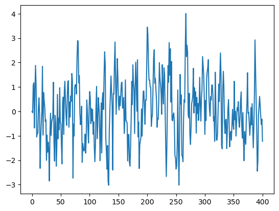

As in other languages, the variables occuring within Python functions have local scope. For example, if we attempt to access the variable drift that we used inside ornstein_uhlenbeck_process, we will get an error.

print(drift) # this will fail because drift is not defined outside of the function

---------------------------------------------------------------------------
NameError                                 Traceback (most recent call last)
Cell In[20], line 1
----> 1 print(drift) # this will fail because drift is not defined outside of the function

NameError: name 'drift' is not defined

As we have seen before, we can use the help functions to check the docstring that we wrote for our function.

help(ornstein_uhlenbeck_process)

Help on function ornstein_uhlenbeck_process in module __main__:

ornstein_uhlenbeck_process(x, alpha=0.1, sigma=1.0, dt=1.0)
    One step for the dynamics of a particle in a harmonic potential, with Brownian noise

    Equivalent to an AR(1) process with alpha = 1

    Args:
        x (float): The current position of the particle
        alpha (float): The spring constant
        sigma (float): The amplitude of the random noise

    Returns:
        float: The position of the particle at the next time step

We can also use the help function to get information about functions we imported from elsewhere.

help(random.gauss)

Help on method gauss in module random:

gauss(mu=0.0, sigma=1.0) method of random.Random instance
    Gaussian distribution.

    mu is the mean, and sigma is the standard deviation.  This is
    slightly faster than the normalvariate() function.

    Not thread-safe without a lock around calls.

type(ornstein_uhlenbeck_process) # type check

function

print(dir(random.gauss)[:10])

['__call__', '__class__', '__delattr__', '__dir__', '__doc__', '__eq__', '__format__', '__func__', '__ge__', '__get__']

Conditional halting of a process¶

In our implementation of the Ornstein-Uhlenbeck process, we run the process for a fixed number of timesteps. However, we might be interested in simulating a trapped particle until the particle escapes by crossing some barrier. In this case, we want a loop that terminates not when a fixed number of iterations is reached, but rather when some condition is met. In this case, we want to use a while loop

# We import Python's linear algebra library, which is used to 
import numpy as np

# set pseudorandom seed
# random.seed(5)

all_steps = [0]
while abs(all_steps[-1]) < 3:
    all_steps.append(
        ornstein_uhlenbeck_process(all_steps[-1], alpha=0.1, sigma=0.5)
    )

plt.figure()
plt.plot(np.arange(len(all_steps)), all_steps)
plt.xlabel('Time step')
plt.ylabel('Position')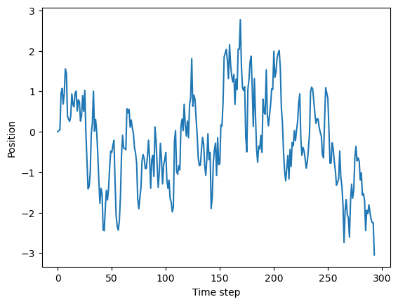

First passage time distributions¶

Our modified Ornstein-Uhlenbeck process runs until the particle crosses a fixed barrier. We can repeat this process many times, and observe the distribution of times it takes for the particle to cross the barrier. In physics, the first-passage time distribution is the probability distribution of the times it takes for a stochastic process to first reach a certain value.

We can think of our simulation as probing a distribution of outcomes. Across many experiments on an optical trap with stiffness $\alpha$ and noise amplitude $\sigma$ , how long do we expect to trap the particle?

Another example where first passage time distributions are useful is in the study of chemical reactions. Oftentimes, reactants must first reach a certain energy threshold before they can react. The distribution of times it takes for the reactants to reach this threshold is the first passage time.

## now run a simulation with many trajectories to get the distribution of first-passage times
all_fpt_durations = []
for i in range(1000): # number of experiments
    all_steps = [0]
    while abs(all_steps[-1]) < 3:
        all_steps.append(ornstein_uhlenbeck_process(all_steps[-1], alpha=0.3, sigma=0.5))

    all_fpt_durations.append(len(all_steps))

plt.figure()
plt.hist(all_fpt_durations, bins=50);
plt.xlabel('First-passage time')
plt.ylabel('Count')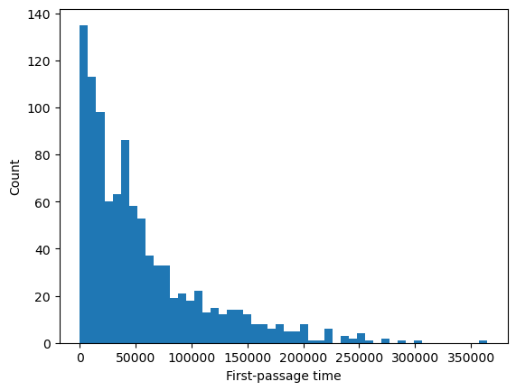

Python functions are objects¶

We can pass Python functions to other functions, as if they were any other variable. Below, we’ll use lambda functions to define two versions of an Ornstein-Uhlenbeck process with different stiffnesses, as well as a Weiner process (the case where $\alpha=0$ ) and random jumps.

# Define several stochastic processes with constant variance 1.0 and varying stiffness
ornstein_uhlenbeck_process_wide = lambda x: x - 0.05 * x + random.gauss(0, 1)

ornstein_uhlenbeck_process_tight = lambda x: x - 0.5 * x + random.gauss(0, 1)

wiener_process = lambda x: x + random.gauss(0, 1)

random_walk = lambda x: random.gauss(0, 1)

Next, we will define a function that will take a given stochastic process as an argument, and return the first passage time distribution.


def first_passage_time(process, n_sim=10000, xc=3):
    """
    Given a random process, perform n_sim simulations and return the durations

    Args:
        process (callable): a function that takes a single argument and returns a single value
        n_sim (int): number of simulations to run
        xc (float): the crossing threshold for the first passage time

    Returns:
        list: durations of the first passage times
    """
    all_fpt_durations = []
    for i in range(n_sim):
        all_steps = [0]
        while np.abs(all_steps[-1]) < xc:
            all_steps.append(process(all_steps[-1]))

        all_fpt_durations.append(len(all_steps))

    return all_fpt_durations

help(first_passage_time)

Help on function first_passage_time in module __main__:

first_passage_time(process, n_sim=10000, xc=3)
    Given a random process, perform n_sim simulations and return the durations

    Args:
        process (callable): a function that takes a single argument and returns a single value
        n_sim (int): number of simulations to run
        xc (float): the crossing threshold for the first passage time

    Returns:
        list: durations of the first passage times

We will now use this function to calculate the first passage time distribution for a stiff and wide Ornstein-Uhlenbeck processes.

# Generate the first passage time distributions
fpt_times_tight = first_passage_time(ornstein_uhlenbeck_process_tight)
fpt_times_wide = first_passage_time(ornstein_uhlenbeck_process_wide)

plt.figure()
plt.semilogy()
plt.hist(fpt_times_tight, bins=50, alpha=0.5, label='tight', color='b')
plt.hist(fpt_times_wide, bins=50, alpha=0.5, label="wide", color='r')
plt.legend()
plt.title("Stiff vs Wide Ornstein-Uhlenbeck processes")
plt.xlabel("First passage time")
plt.ylabel("Count")


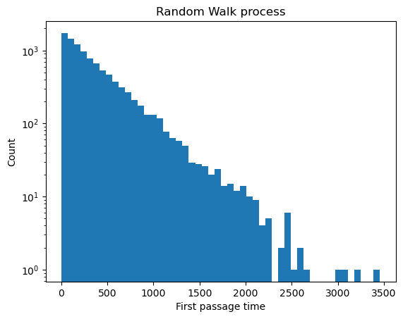
plt.figure()
plt.semilogy()#Make a plot with log scaling on the y-axis
plt.hist(first_passage_time(random_walk), bins=50);
plt.xlabel("First passage time")
plt.ylabel("Count")
plt.title("Random Walk process")

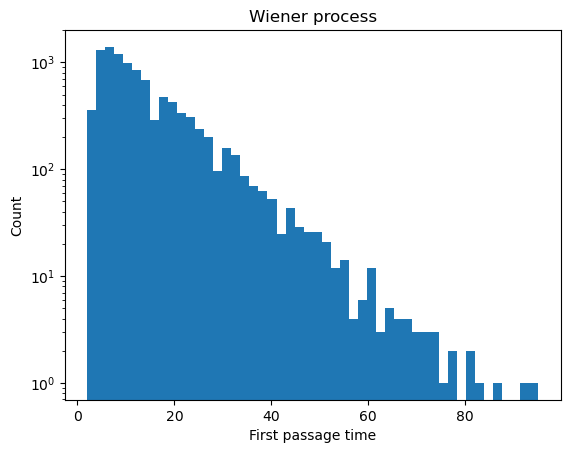
plt.figure()
plt.semilogy()
plt.hist(first_passage_time(wiener_process), bins=50);
plt.xlabel("First passage time")
plt.ylabel("Count")
plt.title("Wiener process")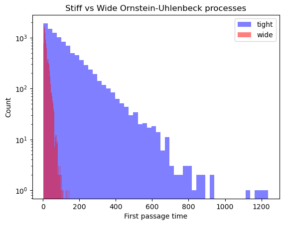

Questions¶

Why does the more strongly-confined process have a narrower first passage time distribution?

What is the simulation showing?¶

The first-passage time distribution of an Ornstein-Uhlenbeck process is difficult to compute analytically, but our simulations suggest that it exhibits a predominantly exponential decay at long times. We can use our results to motivate an analytical approximation for the first-passage time distribution.

We first define the Ornstein-Uhlenbeck process symbolically. We define the drift term to be negative, so the process is mean-reverting.

dx_{t}=-\alpha \,x_{t}\,dt+\sigma \,dW_{t}

(3)

We are using the Ito interpretation of the stochastic differential equation. Notice how when $dW_t$ is zero, we recover a familiar ordinary differential equation. We use this notation because the stochastic term itself cannot be differentiated.

The solution to this equation is:

x_{t}=x_{0}\,e^{-\alpha t} + \sigma \int_{0}^{t}e^{-\alpha (t-s)}\,dW_{s}

(4)

Notice that the second term resembles a Laplace transformation. We can next define a first-passage time function on this interval:

\tau = \inf \{t>0: |x_{t}| \geq x_c\}

(5)

where $x_c$ is the crossing threshold.

The ensemble behavior of the Ornstein-Uhlenbeck process¶

We saw from the first-passage time distribution that the Ornstein-Uhlenbeck process exhibits, on average, an exponential tail when averaged over many realizations. We can also study the ensemble behavior of the process by simulating many realizations of the process and looking for deterministic structures that emerge.

Below, we define a function run_simulation that runs a given stochastic process many times, and returns an array of the results. The resulting array has shape (n_sim, n_tpts), where n_sim is the number of simulations, and n_tpts is the number of time points. The values in the array are the values of the process at each time point for each simulation.

def run_simulation(process, n_sim, n_tpts):
    """
    A function that runs a given stochastic process n_sim times, and returns an 
    array of the results. The process is assumed to be a function that takes a
    single argument (the current value of the process) and returns the next
    value of the process.

    Args:
        process (function): A function that takes a single argument (the current
            value of the process) and returns the next value of the process.
        n_sim (int): The number of simulations to run.
        n_tpts (int): The number of time points to simulate.

    Returns:
        all_simulations (np.ndarray): An array of shape (n_sim, n_tpts) containing
            the results of the simulations. The first axis indexes the simulation
            replicate, and the second axis indexes the time point.
    """

    # Since we know the size of our output in advance, we can pre-allocate the 
    # solution array to avoid the overhead of adding elements to a list
    all_simulations = np.zeros((n_sim, n_tpts))

    for i in range(n_sim):
        for j in range(1, n_tpts):
            all_simulations[i, j] = process(all_simulations[i, j - 1])
    
    return all_simulations



out = run_simulation(ornstein_uhlenbeck_process_wide, 10, 200)
plt.figure(figsize=(8, 4))
plt.plot(out.T);
plt.xlabel('Time')
plt.ylabel('Value')
plt.title('Ensemble behavior of 10 realizations of an Ornstein-Uhlenbeck process')


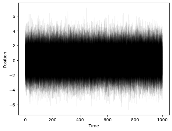
out = run_simulation(ornstein_uhlenbeck_process_wide, 5000, 200)
plt.figure(figsize=(8, 4))
plt.plot(out.T, color='k', alpha=0.005, linewidth=0.5);
plt.xlim(0, out.shape[1])
plt.xlabel('Time')
plt.ylabel('Value')
plt.title('Ensemble behavior of 5000 realizations of an Ornstein-Uhlenbeck process')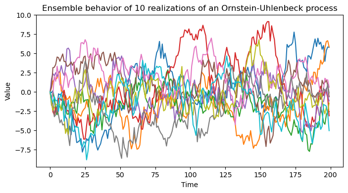

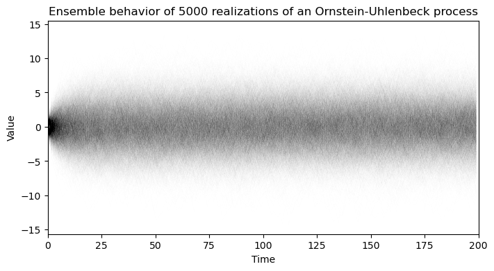
We can see that, while individual realizations of the process vary widely, the ensemble behavior of the process appears to bedeterministic. The ensemble of trajectories initially radiates from the origin at $t=0$ , but they appear to develop a stationary distribution as time progresses.

Understanding the motion of ensembles of particles¶

The Fokker-Planck equation allows us to go from studying the motion of a single particle, $x_{t}$ , to instead studying the motion of a distribution of particles, $p(x, t)$ . Across many random runs of the process, or many random optical trap experiments, $p(x, t)$ tells us how often we expect to find a particle at position $x$ at time $t$ .

The Fokker-Planck equation for an Ornstein-Uhlenbeck process is

\frac{\partial}{\partial t}p(x, t) = \alpha \frac{\partial}{\partial x} \left(x \, p(x, t) \right) + \frac{1}{2}\sigma^{2} \frac{\partial^{2}}{\partial x^{2}}p(x, t)

(6)

Unlike the single-particle stochastic process, the Fokker-Planck equation describes the distribution of trajectories under the process over time. In order to solve this partial differential equation, we need to learn more about how ensembles of trajectories from our process behave.

What does $p(x, t)$ look like? We can find out by inspecting the distribution of positions in the ensemble of trajectories that we just simulated.

plt.figure()
plt.hist(out[:, 1], bins=20, alpha=0.5, label='t=1');
# plt.hist(out[:, 2], bins=20, alpha=0.5, label='t=2');
plt.hist(out[:, 100], bins=20, alpha=0.5, label='t=100');
plt.hist(out[:, -1], bins=20, alpha=0.5, label='t=200');
plt.legend(frameon=False)
plt.xlabel('Final Value')
plt.ylabel('Count')

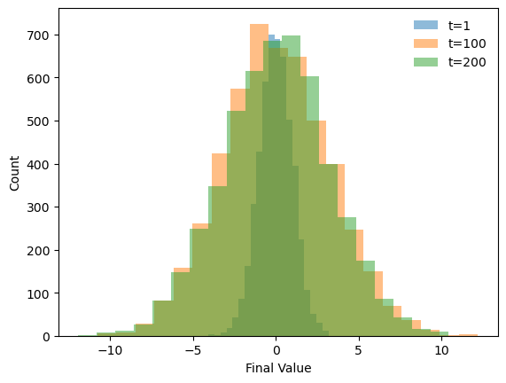
It looks like the long-time limit of the process is a Gaussian distribution with mean at zero and a time-varying variance. This gives an ansatz for the analytical form of $p(x, t)$

p(x, t) = \frac{1}{\sqrt{2\pi \Sigma^2(t)}} \exp \left(-\frac{x^2}{2\,\Sigma^2(t)} \right)

(7)

We next insert this ansatz into the Fokker-Planck equation with an initial condition given by $p(x,0) = \delta(x)$ , because all of our simulations start at the origin.

Simplifying the resulting expression produces an ordinary differential equation for $\Sigma(t)$ ,

\frac{d\Sigma(t)}{dt} = \sigma^2 + 2\alpha \Sigma(t)

(8)

We impose the initial condition $\Sigma(0) = 0$ to find the solution. To avoid singularities, this can be accomplished by setting $\Sigma(0) = \epsilon$ , solving the initial value problem, and then taking the limit $\epsilon \rightarrow 0$ , we arrive at the expression for $\Sigma(t)$ :

\Sigma^2(t) = \frac{\sigma^2}{2\alpha} \left( 1 - e^{-2\alpha t} \right)

(9)

We can see that over a timescale $\tau = 1/(2 \alpha)$ , the variance of the distribution reaches an asymptotic value of $\tilde\Sigma^2 = \sigma^2/(2\alpha)$ . For our tight and wide simulations, $\tau = 1^2 / (2 \cdot 0.5) = 1$ and $\tau = 1^2 / (2 \cdot 0.05) = 10$ , respectively, confirming that our first passage distributions involve timescales beyond the asymptotic limit of the variance. We refer to the stationary Gaussian distribution as $\tilde p(x)$ to distinguish it from the transient time-dependent distribution $p(x,t)$ .

In the asymptotic limit, we can think of the Ornstein-Uhlenbeck process as continuously sampling values from a stationary Gaussian distribution. The probability of success of a given draw is given by the fraction of the distribution that lies above the threshold at $x_c$ at any given time, which is given by $\int_{x_c}^{\infty} \tilde p(x) \, dx$ . In discrete time, if we assume each draw is independent, then the probability of success after $n$ draws is given by the binomial distribution. In continuous time, this process asymptotically approaches an exponential distribution.

Questions¶

What is the probability of success after $n$ draws from a Gaussian distribution with mean 0 and variance $\sigma^2$ ?
Taking the continuous-time limit, what is the probability of success after a time $\tau$ ?
Given the expression for the variance of the Ornstein-Uhlenbeck process described above, what is the probability density function for the first-hitting time $\tau$ ?

Classes and object-oriented programming¶

Classes are abstract Python objects that bundle variables and functions, which are usually called “methods” in this setting. When writing large libraries, classes provide a way to keep track of the state of objects like simulations, and so they are critical for scaling up codebases. Recall how we wrote the function ornstein_uhlenbeck_process to simulate the Ornstein-Uhlenbeck process. We treated the state as the main argument as the function, and we treated the physical parameters of the simulation as optional arguments with default values.

import random
def ornstein_uhlenbeck_process(x, alpha=0.1, sigma=1.0, dt=1.0):
    """
    One step for the dynamics of a particle in a harmonic potential, with Brownian noise

    Equivalent to an AR(1) process with alpha = 1

    Args:
        x (float): The current position of the particle
        alpha (float): The spring constant
        sigma (float): The amplitude of the random noise
        dt (float): The time step

    Returns:
        x_nxt (float): The next position of the particle
    """
    # forcing term
    drift = -alpha * x# * dt

    # stochastic diffusion term
    # random.gauss(0, 1) samples a random value from a normal distribution with mean 0 
    # and variance 1
    diffusion = sigma * random.gauss(0, 1)# * math.sqrt(dt)

    # The OU process is a combination of drift and diffusion
    x_nxt = x + drift + diffusion
    return x_nxt

Class Syntax. All classes have constructor methods named __init__, where Python reserves space for the object and sets the initial values of variables bound to the class, which are called “instance variables” in this setting. When you instantiate a class by assigning a variable, the constructor is called and it builds the object. In our OrnsteinUhlenbeckProcess class, we define the constructor to take two physical parameters describing our simulation, alpha and sigma, and the constructor sets the instance variables self.alpha and self.sigma to the values of the arguments.

Methods are functions that are bound to a class, and which are typically used to modify or query their state. In our OrnsteinUhlenbeckProcess class, we define two methods: step and run_process. The step method takes the current state of the process and returns the next state, and the run_process method takes the number of steps to run the process and returns the trajectory. Even though the class methods are defined within the class, they require their first argument to always be the self keyword, indicating that they will use object-specific variables or methods.

In our OrnsteinUhlenbeckProcess class, we define a method step that evolves the Ornstein-Uhlenbeck process by one step. This method uses the class instance variables self.alpha and self.sigma to compute the next state of the process. These bound functions thus use bound variables without them directly being passed as arguments (they are “bound” to the class through the self keyword). The __init__ method can take standard arguments and keyword arguments, just like any other Python function.

The run_process method does not use any instance variables, but it does use the step method, which it has access to through the self keyword. This function also takes a standard argument, n_steps, which is the number of steps to run the process, as well as an optional keyworkd argument x0, which is the initial state of the process. If this argument is not provided, the process will start at the origin.

import random
class OrnsteinUhlenbeckProcess:
    """
    A class for generating Ornstein-Uhlenbeck processes.

    Parameters:
        alpha (float): spring constant
        sigma (float): noise amplitude
    """

    # Constructor (mandatory for isolated class)
    def __init__(self, alpha=0.2, sigma=1.0):
        self.alpha = alpha
        self.sigma = sigma

    def step(self, x):
        """This method takes the current state of the process and returns the next state"""
        drift = -self.alpha * x
        diffusion = self.sigma * random.gauss(0, 1)
        return x + drift + diffusion

    def run_process(self, n_steps, x0=0):
        """This method runs the Ornstein-Uhlenbeck process for n_steps, starting from x0"""
        all_steps = [x0]
        for i in range(n_steps):
            all_steps.append(self.step(all_steps[-1]))
        return all_steps

    # double underscore methods are special methods to python
    # def __call__(self, x):
        # return self.step(x)

In order to use a class, we have to instantiate it. This differs slightly from built-in types like floats, where Python recognizes the type of the variable and automatically instantiates it. When we instantiate a variable belonging to a class, we pass arguments and set any keyword arguments to the constructor. In our OrnsteinUhlenbeckProcess class, we set the physical parameters of the process during instantiation. These values are now bound to specific instances of the class stored in the variables process1 and process2.

process1 = OrnsteinUhlenbeckProcess(alpha=0.1, sigma=0.5)
print(process1.alpha, process1.sigma)

process2 = OrnsteinUhlenbeckProcess(sigma=0.1, alpha=0.2)
print(process2.alpha, process2.sigma)

0.1 0.5
0.2 0.1

We can query or edit class variables (instance variables) by accessing them directly. Since they are bound to a particular case of the class, we can access them by calling the variable on the instance of the class.

print(f"process2.sigma before change: {process2.sigma}")

process2.sigma = 0.12

print(f"process2.sigma after change: {process2.sigma}")

process2.sigma before change: 0.12
process2.sigma after change: 0.12

We can now use a class method. In this case, we use the run_process method to run the process for a given number of steps. Notice that the class method takes a normal argument, n_steps, but it also implicitly uses the values of the instance variables self.alpha and self.sigma that we set in the constructor and then modified.


traj = process1.run_process(400)
plt.figure()
plt.plot(traj)
plt.xlabel("Time")
plt.ylabel("Position")

traj2 = process2.run_process(400)
plt.plot(traj2)
plt.xlabel("Time")
plt.ylabel("Position")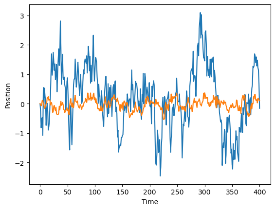

As with any variable or object in Python, we can use the help function to get information about the class.

help(process1)

Help on OrnsteinUhlenbeckProcess in module __main__ object:

class OrnsteinUhlenbeckProcess(builtins.object)
 |  OrnsteinUhlenbeckProcess(alpha=0.2, sigma=1.0)
 |
 |  A class for generating Ornstein-Uhlenbeck processes.
 |
 |  Parameters:
 |      alpha (float): spring constant
 |      sigma (float): noise amplitude
 |
 |  Methods defined here:
 |
 |  __init__(self, alpha=0.2, sigma=1.0)
 |      Initialize self.  See help(type(self)) for accurate signature.
 |
 |  run_process(self, n_steps, x0=0)
 |      This method runs the Ornstein-Uhlenbeck process for n_steps, starting from x0
 |
 |  step(self, x)
 |      This method takes the current state of the process and returns the next state
 |
 |  ----------------------------------------------------------------------
 |  Data descriptors defined here:
 |
 |  __dict__
 |      dictionary for instance variables
 |
 |  __weakref__
 |      list of weak references to the object

help(process1.run_process)

Help on method run_process in module __main__:

run_process(n_steps, x0=0) method of __main__.OrnsteinUhlenbeckProcess instance
    This method runs the Ornstein-Uhlenbeck process for n_steps, starting from x0

Inheritance¶

Inheritance allows you to recycle code by defining abstract classes, then specific refinements of the abstract class known as “subclasses”.

In hierarchical inheritance, the most common type of inheritance, multiple child classes inherit shared methods from a parent class. For example, we might define a generic StochasticProcess class, and then define specific types of stochastic processes like WienerProcess or OrnsteinUhlenbeckProcess as subclasses of the StochasticProcess class. Likewise, we might define a generic NumericalIntegration class, and then define specific types of numerical integration methods like Euler or RungeKutta as subclasses of the NumericalIntegration class.

Another type of inheritance is multiple inheritance, where a child class inherits from multiple parent classes. This often occurs when one wants to access a large number of methods that are associated with multiple parent classes. These usually result in new objects with very different behaviors from other parent. The popular Python library Dysts uses multiple inheritance to create new objects that combine learning model types and problem types.

Image("../resources/inheritance_tree.png")
# Source: https://www.geeksforgeeks.org/types-of-inheritance-python/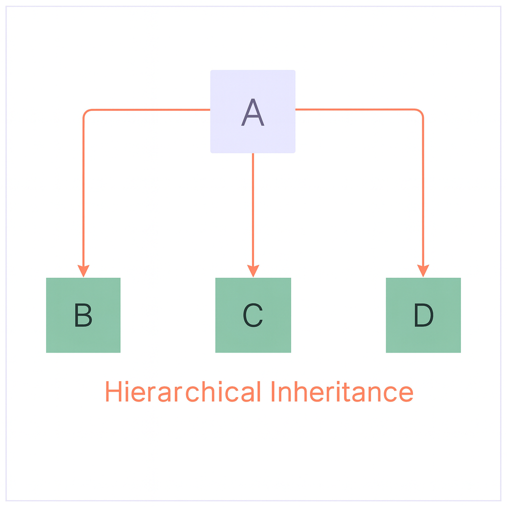

Using Hierarchical Inheritance to define specific types of stochastic processes¶

Let’s see an example of a generic stochastic process class, and then define some specific types of stochastic processes as subclasses of this generic class.

In discrete time, a generic AR(1) (autoregressive, order 1) stochastic process is defined as

X_{t} = f(X_{t-1})

(10)

where $f$ is a function that takes the previous value of the process and returns the current value. This can be a deterministic or a stochastic function. From this generic process we can define a variety of specific types of stochastic processes

Process	Equation	Notes
Generic AR(1)	$X_{t} = f(X_{t-1})$	$f$ can be deterministic or stochastic
Identity	$X_{t} = X_{t-1}$
Wiener	$X_{t} = X_{t-1} + \epsilon$	$\epsilon \sim N(0, \sigma^2)$
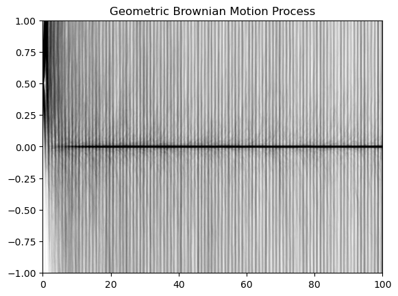
Ornstein–Uhlenbeck	$X_{t} = X_{t-1} - \alpha X_{t-1} + \sigma \epsilon$	$\epsilon \sim N(0, 1), \ \Delta t = 1$
Geometric Brownian Motion	$X_{t} = X_{t-1}(1 + \mu + \sigma \epsilon)$	$\epsilon \sim N(0, 1), \ \Delta t = 1$

Wiener, Ornstein-Uhlenbeck, and Random Walk processes appear throughout natural sciences, and describe the diffusion of chemicals, small particles in fluids, and other phenomena. Geometric Brownian Motion often occurs in finance, as well as other systems where random fluctuations are multiplicative (for example, when they act on percentage cjanges rather than absolute changes).

import numpy as np
class StochasticProcess:
    """
    A base class for stochastic processes.

    Parameters:
        start_val (float): The starting value of the process
        dim (int): The dimension of the process
        noise_level (float): The strength of the noise associated with the process.
        store_history (bool): Whether to store the history of the process
        random_state (int): The random state to use for reproducibility

    """

    def __init__(self, start_val, dim, noise_level=1.0, 
        store_history=True, random_state=None
    ):
        self.dim = dim
        self.start_val = start_val
        self.noise_level = noise_level

        self.store_history = store_history
        self.random_state = random_state

        self.state = start_val
        if self.store_history:
            self.history = [self.state]

    def step(self):
        """
        Subclasses should implement this method. Defaults to Identity process
        """
        # print("Not implemented")
        raise NotImplementedError

    def run_process(self, num_steps):
        """
        Run the process for num_steps.
        """
        np.random.seed(self.random_state)
        for i in range(num_steps):
            self.state = self.step()
            if self.store_history:
                self.history.append(self.state)

        return self.state

ar1 = StochasticProcess(0.1, 1)
print(ar1.noise_level)

hello
1.0

We can learn about the StochasticProcess class by calling the help function on it. We can see that the help function returns the docstring that we wrote above to describe the class, and it also lists the methods that we defined in the class and their docstrings.

help(ar1)

Help on StochasticProcess in module __main__ object:

class StochasticProcess(builtins.object)
 |  StochasticProcess(
 |      start_val,
 |      dim,
 |      noise_level=1.0,
 |      store_history=True,
 |      random_state=None
 |  )
 |
 |  A base class for stochastic processes.
 |
 |  Parameters:
 |      start_val (float): The starting value of the process
 |      dim (int): The dimension of the process
 |      noise_level (float): The strength of the noise associated with the process.
 |      store_history (bool): Whether to store the history of the process
 |      random_state (int): The random state to use for reproducibility
 |
 |  Methods defined here:
 |
 |  __init__(
 |      self,
 |      start_val,
 |      dim,
 |      noise_level=1.0,
 |      store_history=True,
 |      random_state=None
 |  )
 |      Initialize self.  See help(type(self)) for accurate signature.
 |
 |  run_process(self, num_steps)
 |      Run the process for num_steps.
 |
 |  step(self)
 |      Subclasses should implement this method. Defaults to Identity process
 |
 |  ----------------------------------------------------------------------
 |  Data descriptors defined here:
 |
 |  __dict__
 |      dictionary for instance variables
 |
 |  __weakref__
 |      list of weak references to the object

We can now try running the run_process method on the specific ar1 object with just instantiated.

ar1.run_process(100)

---------------------------------------------------------------------------
NotImplementedError                       Traceback (most recent call last)
Cell In[175], line 1
----> 1 ar1.run_process(100)

Cell In[167], line 44, in StochasticProcess.run_process(self, num_steps)
     42 np.random.seed(self.random_state)
     43 for i in range(num_steps):
---> 44     self.state = self.step()
     45     if self.store_history:
     46         self.history.append(self.state)

Cell In[167], line 36, in StochasticProcess.step(self)
     32 """
     33 Subclasses should implement this method. Defaults to Identity process
     34 """
     35 # print("Not implemented")
---> 36 raise NotImplementedError

NotImplementedError:

We can see that our base class StochasticProcess is not very useful by itself, because it does not actually implement a physical model in its step method. We thus need to use inheritance to define subclasses that implement specific types of stochastic processes.

In our implementation, each subclasses implements a different step method that describes the different physical processes. Otherwise, all of thesec subclasses are identical---they initialize the parent class in their own constructor by calling super().__init__. Notice that each subclasse’s __init__ method takes a special *args argument, as well as a special **kwargs argument. In python, *args is a special tuple of arguments that can get passed collectively as arguments to another function, here the __init__ method of the parent class, and **kwargs is a dictionary of keyword arguments that are passed to the parent class constructor. As a result, our subclasses can take the start_val, dim, noise_level, store_history, and random_state arguments, as well as any other arguments that the parent class constructor takes.

## These subclasses are the different types of stochastic processes, and so they 
## inherit methods from the StochasticProcess class.

class IdentityProcess(StochasticProcess):
    """
    The identity process.

    Parameters:
        start_val (float): The starting value of the process
        dim (int): The dimension of the process
        noise_level (float): The strength of the noise associated with the process.
        store_history (bool): Whether to store the history of the process
        random_state (int): The random state to use for reproducibility

    See Also:
        StochasticProcess (parent class): The parent class for all stochastic processes.
    """
    def __init__(self, *args, **kwargs):
        super().__init__(*args, **kwargs)
        ## super() is a function that calls the constructor of the parent class(es) and
        ## passes passes arguments to it

    def step(self):
        return self.state


class WienerProcess(StochasticProcess):
    """
    The Wiener process.

    Parameters:
        start_val (float): The starting value of the process
        dim (int): The dimension of the process
        noise_level (float): The strength of the noise associated with the process.
        store_history (bool): Whether to store the history of the process
        random_state (int): The random state to use for reproducibility

    See Also:
        StochasticProcess (parent class): The parent class for all stochastic processes.
    """
    def __init__(self, *args, **kwargs):
        super().__init__(*args, **kwargs)

    def step(self):
        """Update rule for Brownian motion"""
        return self.state + np.random.normal(0, self.noise_level)

w1 = WienerProcess(0.1, 1, noise_level=0.3)
# w1.dim
help(w1.run_process)

Help on method run_process in module __main__:

run_process(num_steps) method of __main__.WienerProcess instance
    Run the process for num_steps.

traj = w1.run_process(400)
# plt.figure()
# plt.plot(w1.history)
# traj

traj

23.00510858571608

We can also introduce new arguments to the constructor of the subclass, which are unique to the child and are not to the parent. For example, the OrnsteinUhlenbeckProcess class has an additional forcing term in the dynamics, and we can specify the amplitude of this force during instantiation.


class OrnsteinUhlenbeckProcess(StochasticProcess):
    """
    An Ornstein-Uhlenbeck process.

    Parameters:
        start_val (float): The starting value of the process
        dim (int): The dimension of the process
        noise_level (float): The strength of the noise associated with the process.
        store_history (bool): Whether to store the history of the process
        random_state (int): The random state to use for reproducibility
        force_amplitude (float): The amplitude of the deterministic forcing term

    See Also:
        StochasticProcess (parent class): The parent class for all stochastic processes.

    """

    def __init__(self, *args, force_amplitude=0.25, **kwargs):
        super().__init__(*args, **kwargs)
        self.force_amplitude = force_amplitude

    def step(self):
        return self.state + self.force_amplitude * (0 - self.state) + np.random.normal(0, self.noise_level)



class GeometricBrownianMotionProcess(StochasticProcess):
    """
    A geometric Brownian motion process.

    Parameters:
        start_val (float): The starting value of the process
        dim (int): The dimension of the process
        noise_level (float): The strength of the noise associated with the process.
        store_history (bool): Whether to store the history of the process
        random_state (int): The random state to use for reproducibility
        force_amplitude (float): The amplitude of the deterministic forcing term

    See Also:
        StochasticProcess (parent class): The parent class for all stochastic processes.

    """
    def __init__(self, *args, force_amplitude=0.25, **kwargs):
        super().__init__(*args, **kwargs)
        self.force_amplitude = force_amplitude

    def step(self):
        return self.state * (1 + self.force_amplitude + np.random.normal(0, self.noise_level))

Now, let’s try running all of these processes to see that they behave as expected. For each process, we instantiate the child, which then implicity instantiates the parent. We then call the run_process method, which is a method associated with the child that it inherits from the parent. Because step is defined as a placeholder in the parent class, but the child class also implements a step method, the child’s step method overrides the parent’s step method and gets used instead in the call to run_process.

plt.figure(figsize=(10, 8))

identity_process = IdentityProcess(1.0, 1, store_history=True, random_state=14)
identity_process.run_process(100)
plt.plot(identity_process.history, label="Identity")

wiener_process = WienerProcess(0.0, 1, store_history=True, random_state=14)
wiener_process.run_process(100)
plt.plot(wiener_process.history, label="Wiener")

ou_process = OrnsteinUhlenbeckProcess(0.0, 1, store_history=True, random_state=14)
ou_process.run_process(100)
plt.plot(ou_process.history, label="Ornstein-Uhlenbeck")

gb_process = GeometricBrownianMotionProcess(0.5, 1, store_history=True, random_state=14)
gb_process.run_process(100)
plt.plot(gb_process.history, label="Geometric Brownian Motion")



plt.legend()

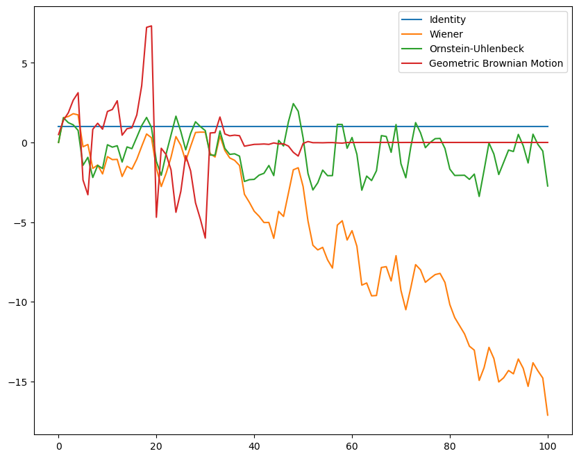
We can see that the Weiner process (standard Brownian motion) and geometric Brownian motion process both appear to be non-ergodic, because the variance and likely other statistical properties of the process appear to change irreversibly over time. The Wiener process tends to move away from the origin, while the geometric Brownian motion process tends either collapse to zero or diverge to infinity.

We can further understand this behavior by simulating many realizations of these processes.

plt.figure()
for i in range(1000): # index is over trajectories
    process = WienerProcess(0.0, 1, store_history=True)
    process.run_process(100)
    plt.plot(process.history, color="black", alpha=0.01)

plt.plot(np.arange(0, 100), np.sqrt(2 * np.arange(0, 100)), color="black", linestyle="--")
plt.plot(np.arange(0, 100), -np.sqrt(2 * np.arange(0, 100)), color="black", linestyle="--")
plt.title("Wiener process")

plt.figure()
for i in range(1000):
    process = GeometricBrownianMotionProcess(0.5, 1, store_history=True)
    process.run_process(100)
    plt.plot(process.history, color="black", alpha=0.01)
plt.xlim([0, 100])
plt.ylim([-1, 1])
plt.title("Geometric Brownian Motion Process")


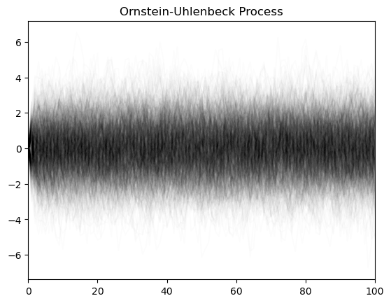
plt.figure()
for i in range(1000):
    process = OrnsteinUhlenbeckProcess(0.0, 1, store_history=True)
    process.run_process(100)
    plt.plot(process.history, color="black", alpha=0.01)
plt.xlim([0, 100])
plt.title("Ornstein-Uhlenbeck Process")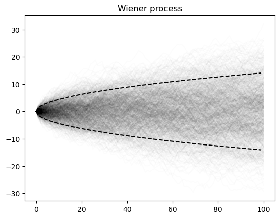

Multiple Inheritance¶

In some cases, we may want to implement Python objects that inherit from multiple parent classes. This can get complicated when there are multiple methods with the same name, like the step method in our StochasticProcess class.

The method resolution order (MRO) defines the order in which Python looks for a method in a hierarchy of classes:

Daughter class methods take precendence over parent class methods. That’s why we were able to override the empty step method in our StochasticProcess class.
However, if two parent classes at the same level of an inheritance hierarchy have the same method, the first one listed in the class definition will take precedence

Image("../resources/multiple_inheritance.png")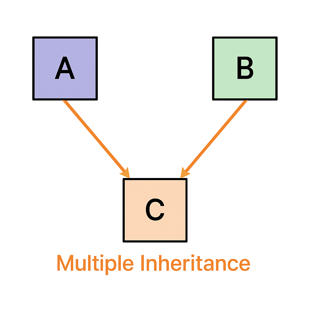

Here’s a minimal example of multiple inheritance in Python. Notice that, since we don’t have any arguments for the constructor, we don’t need to explicitly write an __init__ method in the parent or child, and the child doesn’t need to call the parent’s __init__ method with super().


class A:
    def print_name(self):
        print("Ernest")

class B(A):
    def print_name(self):
        print("Amelia")

    def print_another_name(self):
        print("Blue")

class C(A):
    def print_name(self):
        print("Ferdinand")

class D(C, B):
    pass

# a = A()
# a.print_name() 

# b = B()
# b.print_name() 

# c = C()
# c.print_name()

d = D()
d.print_name()

Ferdinand

We can use this same idea to implement a base class for halting processes, which is a stochastic process that halts when a threshold is reached. The HaltingProcess class is a parent class that defines a step method that must be implemented by the child classes. It also implements a run_halting_process method that runs the halting process until a threshold is reached, or until a certain maximum number of steps is reached. Notice that we use a for loop instead of a while loop. This helps prevent infinite loops. In order to exit early from the for loop, we use the break statement.

class HaltingProcess:
    """
    A base class for halting processes.
    
    Parameters
        threshold (float): The threshold at which the process halts
    """
    def __init__(self, threshold):
        self.threshold = threshold
        # self.store_history = True

    def step(self):
        """
        Subclasses or sibling classes should implement this method
        """
        raise NotImplementedError

    def run_halting_process(self, max_iter=1000):
        """
        Run a halting process, which is a stochastic process that halts when a threshold 
            is reached. If the threshold is not reached after max_iter, then the process
            is halted and the last value is returned.
        """
        np.random.seed(self.random_state)
        for i in range(max_iter):
            self.state = self.step()

            if np.abs(self.state) > self.threshold:
                self.halt_time = i
                break
                # The break statement exits the for loop and stops the simulation
                # before max_iter is reached

            if self.store_history:
                self.history.append(self.state)

        return self.state

We can now implement two child glasses with two parents each. The BrownianHaltingProcess class inherits from both the WienerProcess and the HaltingProcess classes. The OUHaltingProcess class inherits from both the OrnsteinUhlenbeckProcess and the HaltingProcess classes. In our case, the child only inherits one relevant method from each parent: it inherits the step method from the WienerProcess and the HaltingProcess classes, and it inherits the run_halting_process method from the HaltingProcess class.

Question: What would happen if we reverse the order of the parent classes in the definition of the `BrownianHaltingProcess` and `OUHaltingProcess` classes?¶


class BrownianHaltingProcess(WienerProcess, HaltingProcess):
    # The order matters here

    def __init__(self, start_val, threshold, dim=1, **kwargs):
        HaltingProcess.__init__(self, threshold)
        WienerProcess.__init__(self, start_val, dim, **kwargs)
        # The order does not matter here




class OUHaltingProcess(OrnsteinUhlenbeckProcess, HaltingProcess):
    # The order matters here

    def __init__(self, start_val, threshold, dim=1, **kwargs):
        HaltingProcess.__init__(self, threshold)
        OrnsteinUhlenbeckProcess.__init__(self, start_val, dim, **kwargs)
        # The order does not matter here

plt.figure()
for i in range(300):
    model = BrownianHaltingProcess(0.0, 20.0, 1, store_history=True)
    model.run_halting_process()
    plt.plot(model.history, color="black", alpha=0.05)
plt.xlabel("Time")
plt.ylabel("Position")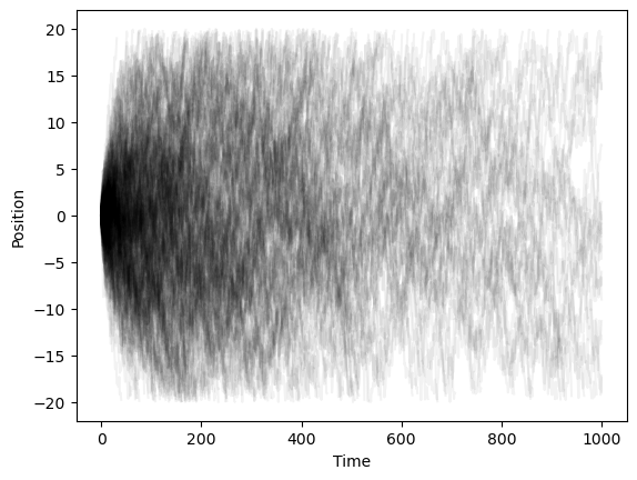


plt.figure()
for i in range(300):
    model = OUHaltingProcess(0.0, 20.0, store_history=True)
    model.run_halting_process()
    plt.plot(model.history, color="black", alpha=0.05)
plt.xlabel("Time")
plt.ylabel("Position")

Some other useful built-ins functions for iterables¶

When we want to iterate over two or more arrays at the same time, we can use the zip function to pair their values together. This can be more concise than using a for loop and then indexing into each of the arrays. Likewise, we can use the enumerate function to iterate over an array and get both the index and the value at each step.

# enumerate provies a tuple of index and value
diffusivities = [0.1, 0.3, 0.6, 0.9]

weiner_process = lambda n, sigma: np.cumsum(np.random.normal(0, sigma, n))
blue = np.array([0.372549, 0.596078, 1])
for i, sigma in enumerate(diffusivities):
    plt.plot(weiner_process(500, sigma), color=blue * (1 - i / len(diffusivities)))
    plt.title(f"Diffusivity {sigma}")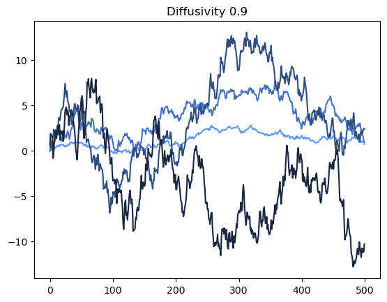

# zip pairs values together
diffusivities = [0.1, 0.3, 0.6, 0.9]

weiner_process = lambda n, signma: np.cumsum(np.random.normal(0, signma, n))
colors = np.array([0.372549, 0.596078, 1]) * (1 - np.arange(0, 1, 0.25)[:, None])
for color, sigma in zip(colors, diffusivities):
    plt.plot(weiner_process(500, sigma), color=color)
    plt.title(f"Diffusivity {sigma}")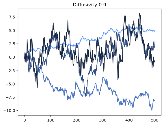

Generators¶

Generators are functions with an internal “state” that serves as a memory. Conceptually, they serve as an intermediate between functions (stateless) and custom objects (stateful). Generators are particularly useful when you don’t want to store an entire array in memory, but still want to iterate over a sequence of values. This is sometimes called a “lazy evaluation” of a sequence, because the values are computed on-the-fly as the generator is iterated over, rather than being computed and stored in advance of the iteration.

def weiner_process(x, max_iter=100):
    for i in range(max_iter):
        yield x + np.random.normal(0, 1)

# next causes the generator to run and then stop when the next yield is reached
process = weiner_process(0)
for i in range(10):
    print(next(process))

1.3047580924456652
-0.05729797829739105
0.5517854029444775
-0.7233012910563584
1.5684284787181064
0.7524096043633353
-1.2311972149145427
0.6348516602027625
-0.3477898301057568
-0.028658650890176128

References¶

Martin, R. J., Kearney, M. J., & Craster, R. V. (2019). Long- and short-time asymptotics of the first-passage time of the Ornstein–Uhlenbeck and other mean-reverting processes. Journal of Physics A: Mathematical and Theoretical, 52(13), 134001. 10.1088/1751-8121/ab0836

Chapters

An Introduction to Python for Scientific Computing

Chapters

Vectorization and arrays: Period-doubling bifurcations and the Mandelbrot Set